Adversarial Examples in Vision

Deep learning models can be confidently fooled into misclassifying images by adding imperceptibly small, carefully crafted noise vectors to the original pixels.

By adding carefully calculated, imperceptible noise to an image, an adversarial attack can force a highly accurate neural network to confidently misclassify a panda as a gibbon.

Why Does This Exist?

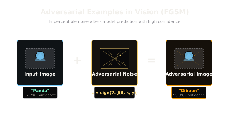
Despite their incredible accuracy on standard benchmarks, deep neural networks are fundamentally vulnerable to highly targeted, visually imperceptible perturbations. Researchers discovered that you could take an image correctly classified as a panda, add a tiny amount of mathematically crafted noise, and cause the model to classify it as a gibbon with 99% confidence. This exists because neural networks operate in high-dimensional spaces where tiny shifts along specific gradient directions can push an input across a decision boundary, exposing a critical flaw in deploying vision models in security-critical environments like autonomous driving or facial recognition.

Think of It Like This

An optical illusion for a machine

When a human looks at an optical illusion, specific patterns of light trick our visual cortex into seeing motion where there is none, or a spiral where there are only concentric circles. We know it's a trick, but our brain processes it incorrectly anyway. Adversarial examples are optical illusions designed specifically for a neural network. By understanding exactly how the network processes pixels, an attacker can arrange a pattern of noise that perfectly triggers the "gibbon" neurons, completely drowning out the actual "panda" visual signal that the human eye sees.

How It Actually Works

Adversarial examples exploit the gradients of the model itself. Instead of updating the model's weights to minimize loss (which is how training works), an attack updates the input image to maximize the loss, keeping the weights frozen.

1. Define the objective: Start with a trained model, an input image $x$ , and its true label $y$ . We want to find a perturbation $\eta$ such that the model misclassifies $x + \eta$ , subject to the constraint that $\eta$ is imperceptible (usually bounded by an $L_\infty$ norm, meaning no pixel changes by more than a small amount $\epsilon$ ).

2. Fast Gradient Sign Method (FGSM): The simplest attack calculates the gradient of the loss with respect to the input pixels. It then takes a small step in the direction of the gradient to maximize the loss.

$\eta = \epsilon \cdot \text{sign}(\nabla_x J(\theta, x, y))$

3. Applying the noise: We add this $\eta$ to the original image: $x' = x + \eta$ . Because $\epsilon$ is very small, the change is invisible to the human eye, but because it aligns perfectly with the model's highest-sensitivity directions across all dimensions simultaneously, it drastically changes the final logits.

4. Targeted vs. Untargeted Attacks: An untargeted attack just tries to make the model predict anything other than the true class. A targeted attack optimizes the input to maximize the probability of a specific, chosen incorrect class.

Code

1import torch2
3def fgsm_attack(image, epsilon, data_grad):4    # Collect the element-wise sign of the data gradient5    sign_data_grad = data_grad.sign()6    7    # Create the perturbed image by adjusting each pixel of the input image8    perturbed_image = image + epsilon * sign_data_grad9    10    # Adding clipping to maintain valid pixel range [0,1]11    perturbed_image = torch.clamp(perturbed_image, 0, 1)12    13    return perturbed_image14
15# Inside an evaluation loop:16# image requires_grad to compute gradients w.r.t pixels17image.requires_grad = True18
19# Forward pass20output = model(image)21loss = criterion(output, target)22
23# Zero all existing gradients24model.zero_grad()25# Calculate gradients of model in backward pass26loss.backward()27
28# Collect the gradient of the input image29data_grad = image.grad.data30
31# Call FGSM Attack32perturbed_data = fgsm_attack(image, epsilon=0.05, data_grad=data_grad)33
34# Re-classify the perturbed image35perturbed_output = model(perturbed_data)36# -> confidently incorrect prediction

Watch Out For

Assuming human perception equals model perception

It is tempting to think that if an image looks completely normal to you, a highly accurate model will process it normally. Models learn heavily from high-frequency texture features, whereas humans rely on shape. Therefore, tiny changes to textures that humans completely ignore can dominate the model's feature maps.

Relying on simple defenses

Defenses like blurring the image, reducing precision, or adding random noise during inference can often be easily bypassed by slightly stronger or more adaptive attacks (like Expectation over Transformation). Truly robust models require computationally expensive techniques like Adversarial Training, where adversarial examples are continuously generated and included in the training batches.

The Quick Version

Adversarial examples are inputs carefully crafted to fool machine learning models.
They are created by adding tiny, imperceptible perturbations to a normal input.
These perturbations are found by calculating the gradient of the loss with respect to the input pixels (e.g., FGSM).
They reveal that deep learning models rely on fragile, non-robust features that align with the dataset but not with human perception.
Defending against them is an ongoing, difficult research problem, primarily addressed through adversarial training.