Frequency Domain Image Processing

Instead of viewing an image as a grid of pixels, frequency domain processing treats it as a sum of 2D sine and cosine waves, allowing us to easily filter out noise or isolate specific patterns.

The Fourier Transform converts a spatial image into its frequency domain representation, where the center represents low frequencies (broad shapes) and the edges represent high frequencies (sharp details and edges).

Why Does This Exist?

When you look at an image in the spatial domain (its raw pixels), certain problems are notoriously difficult to solve. For example, if a photograph is corrupted by a repeating striped pattern (like interference on an old TV), attempting to remove it pixel by pixel without destroying the underlying image is nearly impossible.

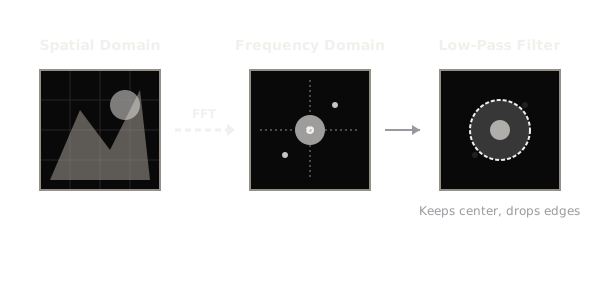
The frequency domain provides an entirely different perspective. By breaking the image down into its constituent wave frequencies, global patterns become isolated points. A repeating stripe that covers the entire image in the spatial domain turns into a single bright dot in the frequency domain. You can simply erase that dot, convert the image back, and the interference vanishes flawlessly.

Think of It Like This

A musical chord vs. sheet music

Imagine you hear a complex chord played on a piano (the spatial domain image). Trying to remove just one out-of-tune string by listening to the combined sound is incredibly hard because the notes are all mixed together.

However, if you transcribe that chord into sheet music (the frequency domain), you can clearly see the individual notes that make up the sound. To fix the chord, you just erase the bad note on the paper and have someone play it again. The Fourier Transform is the tool that transcribes the image into its "sheet music" of frequencies.

How It Actually Works

The 2D Fourier Transform

Any image can be perfectly mathematically reconstructed by adding together many 2D sine and cosine waves of different frequencies, amplitudes, and directions. The Discrete Fourier Transform (DFT)—typically computed using the Fast Fourier Transform (FFT) algorithm—performs this conversion.

Low Frequencies: Represent areas of the image where the pixel values change slowly, such as the smooth sky or a solid wall. These provide the general shape and contrast of the image.
High Frequencies: Represent areas where pixel values change rapidly, such as edges, fine textures, or sharp noise.

The Frequency Spectrum

When you visualize the frequency domain of an image, you get a 2D spectrum plot (often shifted so the lowest frequencies are exactly in the center).

The center is the brightest spot, representing the DC component (the average overall brightness of the image).
As you move outward from the center, you encounter higher and higher frequencies.
A bright spot far from the center indicates a strong repeating pattern or sharp edges oriented in a specific direction.

Filtering in the Frequency Domain

Processing an image in this domain involves three steps:

Transform the image into the frequency domain using the 2D FFT.
Multiply the frequency spectrum by a filter mask.
Apply the Inverse Fast Fourier Transform (IFFT) to convert back to the spatial domain.

Common filters include:

Low-pass filters: Block high frequencies (the outer regions) while letting low frequencies (the center) pass. This blurs the image and reduces noise.
High-pass filters: Block low frequencies and let high frequencies pass. This enhances edges and fine details while stripping away smooth backgrounds.
Band-reject / Notch filters: Target specific points in the spectrum to remove repeating periodic noise.

Code

1import numpy as np2import matplotlib.pyplot as plt3from scipy.fftpack import fft2, ifft2, fftshift, ifftshift4from skimage import color, data5
6# Load a grayscale image7image = color.rgb2gray(data.camera())8
9# 1. Compute 2D Fourier Transform and shift low frequencies to the center10f_transform = fft2(image)11f_shift = fftshift(f_transform)12
13# Display the magnitude spectrum (log scale for visibility)14magnitude_spectrum = 20 * np.log(np.abs(f_shift))15
16# 2. Create a Low-Pass Filter (a circular mask)17rows, cols = image.shape18crow, ccol = rows // 2, cols // 219radius = 3020
21# Create a grid of distances from the center22x, y = np.ogrid[:rows, :cols]23mask_area = (x - crow)**2 + (y - ccol)**2 <= radius**224
25# Apply the mask: keep center, zero out outer frequencies26f_shift_filtered = f_shift.copy()27f_shift_filtered[~mask_area] = 028
29# 3. Inverse transform back to the spatial domain30f_ishift = ifftshift(f_shift_filtered)31image_filtered = np.abs(ifft2(f_ishift))32
33print(f"Original std dev: {image.std():.2f}")             # -> Original std dev: 0.2234print(f"Filtered (blurred) std dev: {image_filtered.std():.2f}") # -> Filtered (blurred) std dev: 0.17

Watch Out For

Ringing artifacts (The Gibbs Phenomenon)

If you use a hard filter mask (like a perfect circle of 1s and 0s, known as an Ideal Filter) in the frequency domain, the sharp cutoff will cause ripple-like waves to appear around the edges in the reconstructed image. This is called ringing. To prevent this, use a filter with a smooth transition, such as a Gaussian or Butterworth filter.

The Quick Version

The frequency domain treats an image as a combination of 2D sine and cosine waves rather than a grid of pixels.
The 2D Fourier Transform converts an image into a frequency spectrum where the center represents smooth shapes (low frequencies) and the edges represent sharp details (high frequencies).
Filtering is done by simply zeroing out or scaling specific regions in the frequency spectrum before transforming back to the spatial domain.
Low-pass filters blur an image by removing high frequencies; high-pass filters extract edges by removing low frequencies.
It is uniquely suited for removing periodic noise (like stripes) that is impossible to isolate in the spatial domain.