Image Transformations and Homography
Learn how linear algebra powers resizing, rotating, and skewing images in computer vision, and understand homography for perspective projection.
Why Does This Exist?
In computer vision, the cameras that capture images are rarely perfectly aligned with the objects they are viewing. If a camera takes a picture of a document from an angle, the document appears skewed or distorted, turning a rectangle into a trapezoid. If we want our algorithms to read that document, we first need a reliable, mathematical way to "flatten" it out. The same applies to simpler edits like rotating a photograph, resizing a thumbnail, or shifting an object's position. All these spatial modifications rely on geometric image transformations.
Image transformations exist to project pixels from one coordinate system to another. This is the cornerstone of tasks ranging from basic photo editing to complex augmented reality and panoramic image stitching. Without mathematical transformations to align and distort pixels systematically, our models would lack spatial reasoning about camera angles and perspectives, treating a tilted square as an entirely different shape than a straight one. By formalizing these transformations mathematically, computer vision pipelines can standardize their inputs, correct lens distortions, and align multiple images taken from slightly different viewpoints.
Whenever your smartphone stitches together a panorama, it relies heavily on image transformations. The phone calculates how the camera moved between each snapshot and applies a specific mathematical mapping to warp the images so they overlap perfectly. Similarly, in medical imaging, scans taken at different times or from different machines must be spatially registered, meaning one image is transformed to perfectly overlay the other for accurate comparison. Thus, the existence of transformations provides the essential spatial glue that ties disparate images back to real-world physical geometry.
Think of It Like This
Stretching rubber over a frame
Think of an image as a flexible rubber sheet with a picture drawn on it.
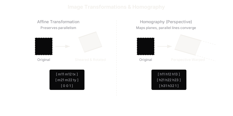
Basic affine transformations (like scaling or rotating) are like stretching the rubber sheet uniformly, rotating it, or moving it around the table. The parallel lines on the drawing always stay parallel—a square might become a skewed parallelogram, but it won't taper. No matter how you stretch it, a grid drawn on the rubber sheet remains a grid with straight lines that never intersect.
A homography, or perspective transformation, is like taking that rubber sheet and tilting it away from you into the third dimension, then taking a photo of it. Parts of the drawing that are further away will look smaller, and parallel lines will now seem to converge in the distance. Homography gives you the mathematical rules to "un-tilt" that sheet back to flat. It allows you to model exactly how light rays from that tilted sheet strike the camera lens, giving you the power to reverse the process mathematically.
How It Actually Works
At its core, a geometric transformation maps each pixel coordinate in the original source image to a new coordinate in the destination image. Because iterating through millions of individual pixels in Python loops is painfully slow, computer vision libraries rely on linear algebra to perform these mappings via highly optimized matrix multiplication.
1. Affine Transformations
Affine transformations include translation (shifting), scaling (resizing), rotation, and shearing. The crucial property of an affine transformation is that it preserves collinearity (straight lines remain straight) and parallelism (parallel lines remain parallel). A rectangle might turn into a parallelogram, but it will never turn into a trapezoid.
To represent all affine transformations uniformly, we use a transformation matrix . We represent pixel coordinates in homogeneous form by appending a to the coordinate vector, resulting in . This neat mathematical trick allows us to encode translation (which is an addition operation) as a multiplication operation alongside scaling and rotation.
In this matrix, and control the rotation, scaling, and shearing effects, while and dictate the translation along the x and y axes. Because the last row is implicitly understood as , an affine matrix has 6 degrees of freedom. You need exactly three pairs of corresponding points between a source and a target image to calculate an unknown affine transformation matrix.
2. Perspective Transformations (Homography)
While affine transformations keep parallel lines parallel, perspective transformations do not. A homography represents the projection of a planar surface from one camera perspective to another. It maps planes to planes, and requires a transformation matrix .
To get the actual 2D coordinates in the new image plane, we must divide the resulting and values by the scaling factor :
This critical division by is precisely what creates the perspective effect, making objects shrink as they recede into the distance. A homography matrix contains 8 degrees of freedom. Since the matrix can be multiplied by any non-zero scalar value without changing the final 2D projection (due to the division by ), is typically normalized and set to 1. To calculate a homography matrix between two planes, you need at least four corresponding point pairs.
In practice, to stitch two photos together, an algorithm like SIFT or ORB first finds dozens of matching feature points between the two images. It then uses an algorithm called RANSAC to aggressively discard incorrect matches (outliers) and calculate the optimal homography matrix from the remaining correct points, allowing one image to be perfectly warped into the perspective of the other.
3. Interpolation
When a coordinate is transformed to , the resulting values are almost never perfect integers. For instance, a pixel might land at . Since digital images only exist on a discrete, integer-based grid, we must determine what color or intensity should be assigned to the new coordinate. This mathematical estimation process is called interpolation.
Common interpolation methods vary in speed and quality:
- Nearest-Neighbor: Snaps to the closest integer pixel. Extremely fast, but leads to heavily jagged, blocky edges.
- Bilinear: Takes a weighted mathematical average of the 4 closest pixels surrounding the point. It is the industry standard default due to its excellent balance of speed and smoothness.
- Bicubic: Takes a weighted average of the 16 closest surrounding pixels. It produces the smoothest edges and sharpest details, but is computationally heavier.
Code
Here is a short OpenCV snippet to apply an affine rotation and a perspective homography. Notice how both rely on calculating a matrix first, then calling a dedicated warp function.
import cv2import numpy as np
# Load imageimg = cv2.imread("document.jpg")rows, cols = img.shape[:2]
# 1. Affine Transformation: Rotate by 45 degrees around the centercenter = (cols / 2, rows / 2)# Get a 2x3 affine rotation matrixrotation_matrix = cv2.getRotationMatrix2D(center, angle=45, scale=1.0)# Warp the image using the affine matrixrotated_img = cv2.warpAffine(img, rotation_matrix, (cols, rows))
# 2. Homography: Perspective warp using 4 corresponding pointspts_source = np.float32([[56, 65], [368, 52], [28, 387], [389, 390]])pts_dest = np.float32([[0, 0], [300, 0], [0, 300], [300, 300]])
# Calculate the 3x3 homography matrix (requires 4 points)homography_matrix = cv2.getPerspectiveTransform(pts_source, pts_dest)# Warp the image using the homography matrixwarped_img = cv2.warpPerspective(img, homography_matrix, (300, 300))Watch Out For
The division by zero in perspective
Because homography coordinates must be divided by to map back to 2D space, you will encounter severe distortions, asymptotes, or numeric crashes if your homography matrix pushes to zero for pixels within your image bounds. This often happens if the input points used to calculate the matrix are collinear (all on the same line) or excessively noisy.
Forward vs. Inverse Warping
Most warping algorithms use inverse warping, looping over the destination grid and pulling pixels from the source using the inverse of the matrix . If you try to forward-warp (loop over the source and push pixels to the destination grid), you'll end up with visual "holes" in your target image where no source pixel perfectly landed on an integer coordinate. Always rely on library functions like warpAffine which handle inverse warping natively.
The Quick Version
- Image transformations map pixel coordinates from one space to another using linear algebra matrices, crucial for alignment and distortion correction.
- Affine transformations (using a matrix) handle shifting, scaling, rotating, and shearing. They keep parallel lines parallel and require 3 points to solve.
- Homographies or perspective transformations (using a matrix) handle viewpoint changes where parallel lines may converge, mimicking 3D depth on a 2D plane. They require 4 corresponding points to calculate.
- Calculating transformations requires homogeneous coordinates, a math trick adding an extra to coordinate vectors so translations can be multiplied like rotations.
- Non-integer target coordinates require interpolation (like bilinear or bicubic) to smoothly guess pixel values based on neighboring grid colors.