Kalman Filter Tracking

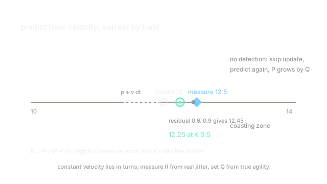
The Kalman filter tracks by predicting where the object should be from its motion, then splitting the difference between that prediction and the new measurement by trust.

Each frame predicts the box forward from velocity, then corrects the prediction toward the detection by the Kalman gain.

Why Does This Exist?

Detections are noisy and intermittent. A detector jitters a box by a few pixels each frame, misses frames entirely during occlusion, and gives no velocity to aim with. Naive tracking that copies the last detection inherits all of that: jittery boxes, lost IDs behind every pillar.

The Kalman filter (1960) is the optimal estimator for linear motion with Gaussian noise, and the workhorse motion model inside classical object tracking pipelines like SORT. It keeps a running belief (position plus velocity) with an uncertainty, predicts it forward each frame, and corrects it with each measurement, weighting prediction against measurement by their relative uncertainties. During occlusion there is no measurement, so it coasts on prediction until the object reappears.

Think of It Like This

Catching a ball with your eyes half closed

You watch a ball arc toward you, blink, and your brain keeps simulating the arc during the blink. When your eyes open, you see the ball slightly off from where you imagined and instantly revise. The longer the blink, the less you trust your simulation; the blurrier your vision, the less you trust your eyes.

Prediction is the simulation during the blink. The measurement is the bleary glimpse. The Kalman gain is the instant revision rule: trust the glimpse more when your simulation is stale, trust the simulation more when your vision is blurry.

How It Actually Works

1. State and prediction

The state holds position and velocity, $x = [p, v]^T$ . Each step predicts forward with the motion model: $p \leftarrow p + v \Delta t$ , $v$ unchanged (constant velocity), while uncertainty $P$ grows by process noise $Q$ . A growing $P$ means "I am getting less sure while coasting."

2. Update by the Kalman gain

A new measurement $z$ arrives with noise $R$ . The gain $K = P / (P + R)$ in the scalar case splits the difference: state $\leftarrow$ prediction $+ K (z - \text{prediction})$ , uncertainty $\leftarrow (1 - K) P$ . Worked: predicted position $12$ , measurement $12.5$ , gain $0.5$ . Updated position $12 + 0.5 \cdot (12.5 - 12) = 12.25$ , exactly halfway because both sides were trusted equally. High $K$ chases measurements; low $K$ rides the model.

3. Coast through occlusion

With no detection, skip the update and predict again. Uncertainty compounds each missed frame, so the gate for matching new detections widens honestly instead of pretending confidence. Particle filters generalize this to non-Gaussian messes where one bell curve cannot hold the belief.

Code

1def kalman_update(pred: float, measure: float, gain: float) -> float:2    return pred + gain * (measure - pred)3
4print(kalman_update(12.0, 12.5, 0.5))  # -> 12.255print(kalman_update(12.0, 12.5, 0.9))  # -> 12.45

Watch Out For

Constant velocity is a lie during maneuvers

The model assumes velocity barely changes, so a sharp turn or sudden stop leaves predictions flying straight while the object is gone. The filter recovers once measurements return, but IDs may already have switched. If tracks swap at every turn, raise process noise $Q$ or move to an interacting-multiple-model setup.

Tuning Q and R by feel

$Q$ (motion surprise) and $R$ (sensor slop) decide everything, and hand-tuned values from one camera fail on another. Measure $R$ from your detector's real jitter on static scenes, then set $Q$ from the fastest accelerations you must follow. Numbers from data beat numbers from vibes.

The Quick Version

The Kalman filter predicts position from velocity, then corrects with the measurement weighted by the gain.
Prediction $12$ with measurement $12.5$ at gain $0.5$ lands exactly at $12.25$ .
Uncertainty grows while coasting, so occlusion handling degrades honestly instead of snapping.
Optimal only for linear motion with Gaussian noise; maneuvers need more process noise.
The motion core of SORT-style trackers; nonlinear cases graduate to particle filters.