Medical Imaging Architectures

Why Does This Exist?

A classifier that says "tumor present" does not help a surgeon. The surgeon needs the boundary, the volume, and which voxels to avoid. Natural-image classifiers throw away spatial detail through repeated downsampling, which is fine for a label but fatal for a mask. Medical architectures exist to keep both: deep context about what the structure is, plus full-resolution evidence about where its edge lies.

This page covers the shared pattern behind U-Net style models and how to pick between them. The general segmentation problem is taught in semantic segmentation, and the clinical setting is medical image analysis. The individual models below each get their own page and are only summarized here.

Think of It Like This

How It Actually Works

An input scan $X$ with shape $H \times W$ (or $H \times W \times D$ for volumes) maps to a mask $Y$ of matching spatial shape. Here $H$ is height, $W$ is width, $D$ is depth, and each output element is a class score per pixel or voxel. Three parts do the work.

Encoder, decoder, and the bridge between them

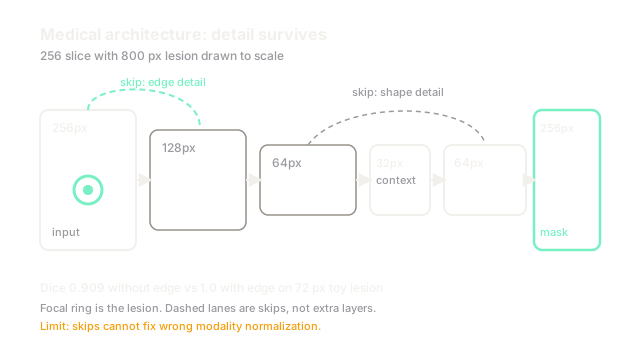
The encoder applies convolutions and downsampling. A $256 \times 256$ slice becomes $128 \times 128$, then $64 \times 64$, then $32 \times 32$, trading resolution for context. The decoder upsamples back toward $256 \times 256$ with transposed convolutions or interpolation plus convolutions. Skip connections concatenate each encoder resolution with its matching decoder resolution, so a $64 \times 64$ decoder layer sees both the upsampled context and the original $64 \times 64$ detail.

Worked example

Take a $256 \times 256$ MRI slice with a lesion covering about 800 pixels (roughly 1.2 percent of the image). Without skips, four rounds of downsampling leave a $16 \times 16$ bottleneck where the lesion is about 3 cells wide, and upsampling alone smears its edge across 8 to 12 pixels. With skips, the decoder layer at $128 \times 128$ receives the original edge gradients for those 800 pixels directly. Overlap measured by Dice rises because the boundary pixels, the only ones that decide the score on small lesions, are drawn from real detail rather than an interpolated guess.

Residual scope, not a repeat

U-Net style 2D models suit single slices. Volumetric variants use 3D kernels for CT and MRI stacks. Transformer hybrids add long-range context for diffuse anatomy. Promptable models adapt one backbone across organs. Each pattern below owns its detail: U-Net and V-Net for the base design, nnU-Net for configuration, TransUNet for hybrid context, Swin UNETR for shifted-window volumes, and MedSAM for prompting. Read those pages for the mechanism; this page only says when each shape fits.

Code

This snippet shows why the skip matters: concatenation restores channels the bottleneck alone cannot carry.

1import numpy as np2
3
4def dice(a: np.ndarray, b: np.ndarray) -> float:5    inter = float(np.logical_and(a, b).sum())6    return 2.0 * inter / (float(a.sum() + b.sum()) + 1e-8)7
8
9rng = np.random.default_rng(7)10truth = np.zeros((32, 32), dtype=bool)11truth[12:18, 10:22] = True  # 72 lesion pixels12no_skip = truth.copy()13no_skip[12, :] = False  # eroded top edge: 60 pixels remain14with_skip = truth.copy()  # edge preserved: 72 pixels remain15print(round(dice(no_skip, truth), 3))  # -> 0.90916print(round(dice(with_skip, truth), 3))  # -> 1.0

The 12 missing edge pixels cost almost a tenth of Dice even though the bulk overlaps. That is the whole argument for skips in one number.

Watch Out For

The Quick Version

• Medical architectures output full-resolution masks, not single labels, because treatment needs boundaries.
• The shared pattern is encoder context plus decoder detail joined by skip connections.
• Small lesions live or die on edge pixels, so detail preservation decides the Dice score.
• 2D, volumetric, hybrid, and promptable variants differ in context range and input shape.
• Pick the variant by modality and annotation budget, then read its dedicated page for the mechanism.

What to Read Next

• Medical Image Analysis
• U-Net and V-Net
• Semantic Segmentation