Core ML

Adam and AdamW

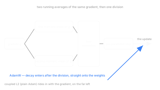
Adam keeps two running averages of the gradient, so every parameter gets its own step size. AdamW moves the weight decay after that division, and took over.

One gradient feeds two running averages, both get bias-corrected, and their ratio becomes a per-parameter step, with AdamW's weight decay entering after that division rather than before it

Why Does This Exist?

One dial controls how far you move. A thousand things need moving by wildly different amounts. One setting can't be right for all of them.

That's the situation on the example we'll carry down the page: fine-tuning a 110-million-parameter text classifier on 20,000 support tickets. Gradients on the embedding layer and gradients on the final classifier head differ in typical magnitude by factors of a thousand. Pick a rate that moves the head sensibly and the embeddings barely budge. Pick one for the embeddings and the head diverges.

Adam is two ideas bolted together to fix that. The first you have: momentum keeps a running average of the gradient so the step follows a consistent direction rather than the latest noisy one. The second is where the per-parameter behaviour comes from.

Think of It Like This

Gain-staging a mixing desk

A mixing desk with a row of channel strips, one per microphone. Each strip has a fader you push, and above it a trim you set from how loud that channel has been running.

Without trim, the faders are useless as a shared control. The kick drum runs hot, so a centimetre of fader is a huge change. The room mic is whisper-quiet, so the same centimetre does nothing.

Set each trim from that channel's own recent level and it changes. Divide the hot channel down, bring the quiet one up, and one centimetre now means the same audible change on every strip.

Faders are the gradient direction. Trims are the second moment.

How It Actually Works

Two averages, updated every step from the same gradient $g_t$ :

m_t = \beta_1 m_{t-1} + (1 - \beta_1) g_t, \qquad v_t = \beta_2 v_{t-1} + (1 - \beta_2) g_t^2

$m_t$ is the first moment, an exponential moving average of the gradient, $\beta_1$ usually 0.9. That's momentum, giving direction. $v_t$ is the second moment, the same average of the squared gradient, $\beta_2$ usually 0.999. No direction, only size: how big this one parameter's gradients have been running.

Dividing by the square root of $v_t$ is where everything comes from. A parameter whose gradients stay tiny has a tiny $\sqrt{v_t}$ , so dividing by it produces a large step; one with large gradients gets scaled down. Every parameter ends up with its own effective rate from its own history, and one global $\eta$ becomes reasonable to set. RMSprop is this second moment alone, without momentum, and it came first.

Bias correction, the part everyone skips

Both averages start at zero. So at step one $m_1 = 0.1 g_1$ — a tenth of the gradient, not the gradient — and $v_1$ is a thousandth of $g_1^2$ . Their own initial value drags them toward zero, and they stay biased until the decay washes it out. Adam divides that away exactly:

\hat{m}_t = \frac{m_t}{1 - \beta_1^{\,t}}, \qquad \hat{v}_t = \frac{v_t}{1 - \beta_2^{\,t}}, \qquad \theta_{t+1} = \theta_t - \eta \frac{\hat{m}_t}{\sqrt{\hat{v}_t} + \epsilon}

The correction is the decay coefficient raised to the step count, subtracted from one. At $t = 1$ that divides $m$ by 0.1 and $v$ by 0.001, recovering unbiased estimates. Because the coefficients differ, the biases wash out at different rates, and the mismatch is what breaks the step size — the numerator recovers in tens of steps, the denominator in thousands. Skip it and the first few hundred steps are the wrong size, and those are the steps that decide where the run goes.

$\epsilon$ , typically $10^{-8}$ , has one job: keep you from dividing by something near zero when a parameter's gradients have been flat. A guard, not a tuning knob. See numerical stability for why it matters more than it looks.

AdamW, and the one line that made it the default

Weight decay in plain Adam is added into the loss as an $L_2$ penalty, so it arrives as part of $g_t$ — and then gets divided by $\sqrt{\hat{v}_t}$ along with everything else. Follow that through. A parameter with large gradients has a large second moment, so its penalty gets scaled down, while one with small gradients gets penalised hard. The strength you set is not the one any individual parameter receives.

AdamW decouples it. The decay is applied straight to the parameters, after the division, as its own term:

\theta_{t+1} = \theta_t - \eta \frac{\hat{m}_t}{\sqrt{\hat{v}_t} + \epsilon} - \eta \lambda \theta_t

$\lambda$ is the decay strength, and now every parameter shrinks by the same fraction per step whatever its gradient history. That's the whole change, and it's why AdamW replaced Adam nearly everywhere.

The plain verdict: AdamW for transformers and most deep models. SGD with momentum stays competitive in vision and sometimes wins outright on a long schedule. Adam's advantage is largest early, when the per-parameter scaling does the most work.

Show Me the Code

Constant gradient, four steps, corrected against uncorrected.

1import numpy as np2
3
4def first_steps(g: float = 0.1, b1: float = 0.9, b2: float = 0.999,5                lr: float = 1e-3, n: int = 4) -> None:6    m, v = 0.0, 0.07    for t in range(1, n + 1):8        m = b1 * m + (1 - b1) * g              # first moment: which way, how consistently9        v = b2 * v + (1 - b2) * g * g          # second moment: how big this parameter's g runs10        raw = lr * m / (np.sqrt(v) + 1e-8)     # both averages still dragged toward zero11        m_hat, v_hat = m / (1 - b1**t), v / (1 - b2**t)12        fixed = lr * m_hat / (np.sqrt(v_hat) + 1e-8)13        print(f"step {t}  uncorrected {raw:.2e}  corrected {fixed:.2e}  off by {raw / fixed:4.2f}x")14
15
16first_steps()17# -> step 1  uncorrected 3.16e-03  corrected 1.00e-03  off by 3.16x18# -> step 2  uncorrected 4.25e-03  corrected 1.00e-03  off by 4.25x19# -> step 3  uncorrected 4.95e-03  corrected 1.00e-03  off by 4.95x20# -> step 4  uncorrected 5.44e-03  corrected 1.00e-03  off by 5.44x

Three to five times too large, and getting worse before it gets better.

Watch Out For

An L2 term in the loss, expected to behave like weight decay

Symptom: you sweep the regularisation coefficient across two orders of magnitude with Adam and validation barely moves. The usual conclusion is that this model doesn't need regularisation.

It's the coupling. Your penalty went in through the gradient, so the second moment rescaled it per parameter, and the number you swept isn't the pressure any parameter felt. Switch to AdamW, where the decay bypasses the division, and re-run the sweep — the curve usually develops a shape. Check what your framework does, too: some optimiser classes take a weight_decay argument that couples, with the decoupled version in a separate class.

The default learning rate on a fine-tuning run

Symptom: fine-tuning on the 20,000 tickets, and validation accuracy drops below the pretrained model's zero-shot score within a few hundred steps, then claws back to something mediocre.

0.001 is Adam's default because it suits training from scratch, where the weights are random and large moves are the point. Adapting pretrained weights is the opposite: they already encode something, and Adam's per-parameter scaling makes those steps larger than the raw gradients suggest. A few hundred steps at 0.001 erases what you were building on. Start two orders of magnitude lower, around $10^{-5}$ , warm up over the first few hundred steps, and check validation before the first epoch ends.

The Quick Version

First moment: a running average of the gradient. Direction, and that's momentum.
Second moment: a running average of the squared gradient. Size, per parameter, and dividing by its square root hands each parameter its own effective rate.
That's what lets one global rate work across layers whose gradients differ a thousandfold.
Bias correction divides by one minus the decay coefficient raised to the step count. Skip it and the first few hundred steps run three to five times too large.
$\epsilon$ stops a division by something near zero. Not a tuning knob.
Adam's $L_2$ penalty rides in through the gradient and gets rescaled by the second moment, so the strength you set isn't the one you get. AdamW applies the decay after the division.
AdamW for transformers and most deep models. SGD with momentum still wins some vision problems.