Core ML

Attention Mechanism

Instead of reading one fixed summary vector, let the decoder look back at every encoder state and weigh each one by how relevant it is to the current step.

Instead of reading one fixed vector, the decoder scores every encoder state, turns the scores into weights that sum to one, and blends the encoder states by those weights at each step

Why Does This Exist?

The sequence-to-sequence architecture has one specific, well-diagnosed wall: every fact about the input sentence has to survive being compressed into a single fixed-size vector before the decoder ever sees it. For a five-word sentence that's rarely a problem. For a 40-word sentence, it is — translation quality on that architecture drops off a cliff past roughly 20 to 30 source tokens, and the drop isn't a training artifact. It's the architecture asking a fixed-size container to hold an unboundedly large amount of information.

Here's the concrete failure researchers were chasing in 2014 and 2015: translating a long sentence, the decoder would nail the first few words, generated while the context vector was still fresh, and then visibly degrade — dropping clauses, repeating phrases, losing track of which source word it was supposed to be rendering next. The bottleneck was measurable in exactly the sentences you'd expect: the long ones.

Think of It Like This

Highlighting a textbook instead of memorizing it first

Recall the earlier analogy for sequence-to-sequence: reading a report once, closing it, and writing a summary purely from memory. Attention is what happens when you're allowed to keep the report open on the desk while you write, glancing back at whichever paragraph is relevant to the sentence you're writing right now.

You don't reread the whole report for every sentence of your summary — you glance at the part that matters for this sentence, weighted by how relevant each paragraph is to what you're currently writing. Write the next sentence, and you might glance somewhere else entirely. Nothing was ever compressed into one fixed memory that had to hold everything; the whole report stays available, and each moment draws on it differently.

How It Actually Works

Score, then weigh, then blend

At each decoder step $t$ , attention runs three operations against every encoder hidden state $e_1, \ldots, e_n$ — not just the last one.

Score. Compare the current decoder state $d_t$ against each encoder state, producing one number per encoder position:

\text{score}(d_t, e_i) = d_t^\top W_a e_i

(This is one common form — dot-product attention, up to a learned matrix $W_a$ . Additive attention runs the two vectors through a small feedforward layer instead; the scoring function varies, the rest of the mechanism doesn't.)

Weigh. Turn the $n$ raw scores into a probability distribution with softmax:

\alpha_{t,i} = \frac{\exp(\text{score}(d_t, e_i))}{\sum_{j=1}^{n} \exp(\text{score}(d_t, e_j))}

Every $\alpha_{t,i}$ is between 0 and 1, and they sum to exactly 1 across all $n$ encoder positions — a genuine probability distribution over "how relevant is each source position, right now."

Blend. Use those weights to combine the encoder states into a context vector for this specific step:

c_t = \sum_{i=1}^{n} \alpha_{t,i} \, e_i

That $c_t$ then feeds into the decoder alongside its own hidden state to produce the next output token.

Why this removes the bottleneck

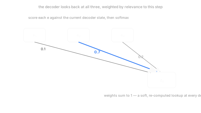
Compare $c_t$ here against the sequence-to-sequence context vector $c$ : the old version was one vector, computed once, used at every decoding step regardless of what was actually being generated. This $c_t$ is recomputed at every single decoder step, and it's a weighted combination of all $n$ encoder states, not a compression of them into a smaller fixed vector. The encoder's full output — every $e_i$ , for every input position — stays available throughout decoding. Nothing about the input has to survive a bottleneck, because there is no bottleneck: the decoder can, in principle, put nearly all of its attention weight on the one encoder position that matters for the word it's producing right now, and different weight entirely for the next word.

The diagram above shows this concretely: decoding position 2 puts weight 0.7 on encoder state $e_2$ , and smaller weights on $e_1$ and $e_3$ . Decoding position 3 would very plausibly redistribute that weight entirely differently — attention isn't fixed once and reused; it's a fresh computation at every step, conditioned on what the decoder is doing right now.

What attention weights actually reveal

Because $\alpha_{t,i}$ is an explicit, inspectable number, attention weights double as a rough diagnostic: plotting them for a translation task typically shows a soft diagonal, with visible off-diagonal spikes exactly where word order differs between the two languages. That interpretability, on top of the accuracy gain, is part of why attention spread so quickly once it worked.

Show Me the Code

Scoring, softmax, and blending, run explicitly rather than fused, against three encoder states and one decoder state.

1import numpy as np2
3
4def softmax(z: np.ndarray) -> np.ndarray:5    e = np.exp(z - z.max())6    return e / e.sum()7
8
9def attend(d_t: np.ndarray, encoder_states: np.ndarray, w_a: np.ndarray) -> tuple[np.ndarray, np.ndarray]:10    scores = encoder_states @ w_a @ d_t          # one score per encoder position11    weights = softmax(scores)                    # sums to exactly 112    context = weights @ encoder_states            # weighted blend of ALL encoder states13    return context, weights14
15
16rng = np.random.default_rng(0)17encoder_states = rng.normal(size=(3, 4))          # 3 source positions, hidden size 418d_t, w_a = rng.normal(size=4), rng.normal(scale=0.3, size=(4, 4))19context, weights = attend(d_t, encoder_states, w_a)20print(np.round(weights, 3))    # -> [0.319 0.354 0.327] — close, none dominant this step21print(np.round(weights.sum(), 6))  # -> 1.0

weights.sum() is exactly 1.0 by construction — that's the softmax, not a coincidence — and context is a genuine weighted average of all three rows of encoder_states, never a copy of just one.

Watch Out For

Forgetting attention weights change every decoder step

It's tempting to think of attention as computing one alignment between source and target sentences, the way a bilingual dictionary aligns words once. It doesn't — $\alpha_{t,i}$ is indexed by $t$ , the current decoder step, precisely because the relevant source position usually shifts as generation proceeds. Caching or reusing attention weights across decoder steps, instead of recomputing the score-softmax-blend sequence fresh each time, silently breaks the entire mechanism: the decoder ends up looking at whatever was relevant to an earlier word for every word after it.

Unscaled dot-product scores collapsing the softmax

As the hidden dimension grows, raw dot-product scores $d_t^\top W_a e_i$ tend to grow in magnitude along with it, and a softmax over large, spread-out scores collapses toward a near one-hot spike — all the weight on a single position, gradients near zero everywhere else. This is exactly the instability that motivated dividing scores by $\sqrt{d_k}$ in the scaled dot-product form used throughout modern attention. If attention weights are consistently near-one-hot from the very first training step, check whether scores need scaling before assuming the model has genuinely learned a sharp alignment.

The Quick Version

Attention lets a decoder look back at every encoder state, at every step, instead of relying on one fixed-size summary vector.
Three operations per step: score each encoder state against the current decoder state, softmax the scores into weights summing to 1, and blend the encoder states by those weights.
The blended context vector is recomputed fresh at every decoder step — it isn't fixed once and reused.
This removes the sequence-to-sequence bottleneck because the full encoder output stays available throughout decoding.
Attention weights are inspectable and typically show a soft, interpretable alignment between output and input positions.