Core ML

Decision Trees

Split the rows on one number, then split each half again. That habit buys rules a dispatcher can read, and costs you any boundary that isn't a staircase.

Three axis-aligned splits carve the feature space into rectangles, so a boundary that runs diagonally can only ever be traced as a staircase

Why Does This Exist?

You've already written a decision tree. Nest a few if-statements — payload over 3 kg, trip over 24 km, don't send it — and that's one, by hand. A learning algorithm only picks the questions, in the order that sorts the data fastest.

You run delivery drones and want to know, before takeoff, whether a flight comes home with charge to spare. Two numbers per flight: payload in kilograms, round-trip distance in kilometres. Six hundred past flights, labelled made it or ran flat.

A linear model would hand you 0.42 × weight + 0.11 × distance, which nobody in dispatch can act on. A tree hands them "over 3.2 kg and over 24 km: hold the flight" — a real advantage, and a distant second reason to care. The first: this is the building block. Random forests, gradient boosting, every tabular winner of the last fifteen years is this object, stacked.

Think of It Like This

A sorting office where every worker reads one gauge

Parcels come down a belt. At the first station a worker glances at one gauge, weight, and pushes each parcel left or right. Two workers downstream read a different gauge and split again. Three stations, four chutes.

A chute is good when almost everything in it is the same kind. That's the whole objective: pick the gauge and cutoff that leave the chutes least mixed.

Now the constraint. Every worker reads one gauge. Nobody may add weight to distance and act on the sum, because that sum isn't a gauge on the wall. So when the rule you need is "weight plus distance under five", the line fakes it with a run of stations, each shaving a corner. Close. Never the diagonal.

How It Actually Works

Picking a split

At a node the algorithm is brute force and unapologetic. Every feature, every cut point between two observed values: split the rows, score how much less mixed the children are, keep the winner, recurse.

"Less mixed" needs a number. Gini impurity is $1 - \sum_k p_k^2$ , where $p_k$ is the share of rows at the node in class $k$ — the chance two rows pulled from the node disagree. Entropy is $-\sum_k p_k \log p_k$ , the average surprise of a label drawn from the node (the derivation). Both sit at zero on a pure node and peak on a 50/50 one, rank splits identically most of the time, and entropy costs a logarithm per candidate — so Gini is the default nearly everywhere. For a numeric target both give way to variance reduction — how much a split shrinks the target's spread in each child.

The score is one subtraction, the parent's impurity minus the row-weighted average of its children's:

\text{gain} = I(\text{parent}) - \frac{n_L}{n}\,I(\text{left}) - \frac{n_R}{n}\,I(\text{right})

$I$ is whichever impurity you chose, $n_L$ and $n_R$ how many rows land left and right, $n$ the parent's count. Those weights are load-bearing: a split that peels three rows into a pure child has earned almost nothing.

Pruning is what makes trees usable

Left alone, the recursion runs until every leaf is pure. On six hundred flights that's hundreds of leaves, several of them housing one flight that had a tailwind.

Pre-pruning refuses to grow: cap the depth, set a minimum rows per leaf, demand a minimum impurity decrease. Almost free, and greedy in the damaging sense — a split that looks worthless alone can set up a good one two levels below, and pre-pruning kills the parent first.

Post-pruning grows the tree out, then collapses branches that didn't pay. Cost-complexity pruning is the principled version — charge for leaves:

R_\alpha(T) = R(T) + \alpha\,|T|

$R(T)$ is the tree's error, $|T|$ its leaf count, $\alpha$ the price per leaf. Raise $\alpha$ from zero and the tree collapses through a predictable sequence of nested subtrees; take the $\alpha$ that wins on cross-validation. One scalar, and depth answers itself.

The staircase

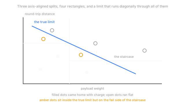
Every split compares one feature against one threshold — a cut perpendicular to an axis. So the regions a tree can produce are always rectangles with sides parallel to the axes.

Your battery limit is not a rectangle. Energy scales with weight and distance together, so the frontier between made it and ran flat runs diagonally. A tree approaches it by stacking steps: cut at 3.2 kg, then cut distance differently on each side, then again. Every extra split halves a step; none tilts one.

That's the inductive bias. Hand a tree a rotated boundary and it spends depth — and therefore variance — on an approximation a single line would have nailed; engineer weight × distance as a feature and it gets there in one split. No scaling needed, mixed types and missing values fine, rotation never. Choose your problems accordingly.

Show Me the Code

One node, scored honestly: every cut point on both features, under both impurities.

1import numpy as np2
3def impurity(y: np.ndarray, kind: str) -> float:4    p = np.bincount(y, minlength=2) / y.size          # class shares at this node5    return float(1 - (p * p).sum()) if kind == "gini" else float(-(p * np.log2(p + 1e-12)).sum())6
7def best_split(x: np.ndarray, y: np.ndarray, kind: str) -> tuple[int, float]:8    cut, best = (-1, 0.0), 0.09    for f in range(x.shape[1]):10        for t in np.unique(x[:, f])[:-1]:             # a cut above the max separates nothing11            lo = x[:, f] <= t12            gain = impurity(y, kind) - lo.mean() * impurity(y[lo], kind) - (1 - lo.mean()) * impurity(y[~lo], kind)13            if gain > best:14                cut, best = (f, float(t)), gain15    return cut16
17flights = np.random.default_rng(0).uniform(0.5, 4.5, (400, 2))  # payload kg, trip in tens of km18home = (flights.sum(axis=1) < 5.0).astype(int)                  # the battery limit is diagonal19g, e = best_split(flights, home, "gini"), best_split(flights, home, "entropy")20print(f"gini cuts feature {g[0]} at {g[1]:.2f}; entropy picks feature {e[0]} at {e[1]:.2f}")21# -> gini cuts feature 0 at 2.61; entropy picks feature 0 at 2.07

Same feature, different threshold. That's the usual disagreement between the two measures, and it washes out once the children get split in turn. The 1e-12 guards the logarithm against a pure child.

Watch Out For

A tree that scores 1.00 on its own training set

Perfect training accuracy is the default for an unpruned tree, not an achievement. The symptom: training accuracy 1.00, validation near a coin flip, no leaf holding more than two rows.

More data won't fix it; the tree grows deeper and isolates the new oddities too. Cap the depth, raise the floor on rows per leaf, or sweep $\alpha$ and let cross-validation choose. Then measure again.

Believing the feature importances your library printed

Impurity-based importance sums how much each feature reduced impurity across the tree. It reads like a ranking of what matters. It's partly a ranking of how many cut points each feature offered — 400 distinct values gets 399 chances to look useful, a binary flag one.

You'll notice when a customer ID or a raw timestamp outranks a feature you know is causal. Permutation importance on held-out data is the honest version: shuffle one column, measure how far validation drops, put it back, repeat. Slower, and it answers the question you asked.

The Quick Version

Search every feature and cut point at each node, keep the split that drops impurity most, recurse.
Gini is $1 - \sum p_k^2$ , entropy is $-\sum p_k \log p_k$ ; they almost always agree and Gini is cheaper. Numeric targets use variance reduction.
Information gain is the parent's impurity minus the row-weighted average of the children's; those weights stop tiny pure leaves looking good.
Pre-pruning stops growth early and is greedy: it can't see a good split two levels down.
Cost-complexity pruning grows out, then prunes to the subtree minimising error plus $\alpha$ per leaf, $\alpha$ from cross-validation.
Axis-aligned splits turn a diagonal frontier into a staircase, and no depth removes it.
A single tree is rarely what you ship — its variance is why every ensemble on this site exists.