Core ML

Depthwise Separable Convolutions

Split one expensive convolution into a cheap per-channel pass and a cheap channel-mixing pass, cutting the parameter count by nearly an order of magnitude.

A standard convolution mixes space and channels in one step; splitting that into a per-channel spatial pass and a separate 1×1 channel-mixing pass does the same job with a fraction of the weights

Why Does This Exist?

Say the target is a phone camera app that detects and blurs faces in the live preview, running entirely on the device — no server round trip, thirty times a second, on a phone's power budget rather than a data center's. A standard convolutional layer that reads 128 channels and writes 256, with a 3×3 kernel, needs 294,912 weights. That's one layer. A real network needs dozens, and every one of those weights is a multiply-and-add the phone's processor has to perform for every pixel, every frame, on a battery.

The wall isn't that this is impossible — plenty of powerful networks exist that size. The wall is that a network built at that cost simply won't run at a usable frame rate on the hardware a phone actually has, and it will drain the battery doing it. Something has to give, and shrinking the network by making it shallower or narrower loses the accuracy the task needs. The fix that MobileNet's authors landed on doesn't remove capability — it rebuilds the convolution itself to do the same job for a fraction of the weight count.

Think of It Like This

Two specialists instead of one generalist

Imagine sorting a warehouse of boxes that need both repositioning on the floor and relabeling with a new inventory code. One generalist worker who does both jobs at once, box by box, needs training and equipment for the full combined task — expensive to hire, expensive to equip.

Split the job instead. One specialist repositions boxes on the floor, full stop, no labeling equipment needed. A second specialist relabels boxes exactly where they already sit, no forklift needed. Neither specialist needs the combined skillset or the combined equipment, and hiring two narrow specialists costs far less than one worker capable of doing both jobs simultaneously — even though the warehouse ends up fully repositioned and fully relabeled either way.

How It Actually Works

What a standard convolution actually pays for

A standard 3×3 convolution reading $C_{in}$ channels and writing $C_{out}$ channels does two things simultaneously, in one set of weights: it looks at a spatial neighborhood (the 3×3 part), and it mixes information across every input channel to produce every output channel (the $C_{in} \times C_{out}$ part). Its parameter count is the product of both: $3 \times 3 \times C_{in} \times C_{out}$ . Both jobs are genuinely necessary — but nothing says they have to be paid for in the same set of weights.

Splitting the two jobs apart

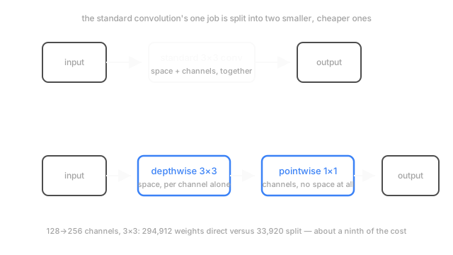
A depthwise convolution does only the spatial part. It applies one small kernel per input channel, independently — a 3×3 filter that looks at channel 1 and only channel 1, a separate 3×3 filter for channel 2 and only channel 2, and so on. No mixing across channels happens here at all; the output has exactly as many channels as the input, each one filtered on its own. Parameter count: $3 \times 3 \times C_{in}$ — no multiplication by $C_{out}$ , because there's no cross-channel mixing to pay for.

A pointwise convolution does only the channel-mixing part. It's a 1×1 convolution — no spatial neighborhood at all, just a weighted combination of the channels present at each individual pixel, mapping $C_{in}$ channels to $C_{out}$ . Parameter count: $C_{in} \times C_{out}$ .

Chain them — depthwise first, pointwise second — and the combined operation reads a spatial neighborhood and mixes channels, exactly like the standard convolution did, just as two smaller steps instead of one combined one. Total parameters: $3 \times 3 \times C_{in} + C_{in} \times C_{out}$ , which is additive where the standard convolution's cost was multiplicative.

The actual savings, computed

For the 128-to-256-channel example this page opened with: a standard 3×3 convolution costs $3 \times 3 \times 128 \times 256 = 294{,}912$ weights. The depthwise-separable version costs $3 \times 3 \times 128 + 128 \times 256 = 1{,}152 + 32{,}768 = 33{,}920$ — about 8.7 times fewer weights for the identical input and output shape. The general reduction factor, for any $C_{out}$ and kernel size $k$ , works out to $\frac{1}{C_{out}} + \frac{1}{k^2}$ of the original cost — the larger $C_{out}$ gets, the closer the savings approach a full $k^2$ -times reduction, because the pointwise step's cost (which doesn't shrink) becomes a smaller share of an already-small total.

What's actually lost

This isn't a free lunch, and it's worth being honest about the trade. A depthwise-separable layer has real structural constraints a standard convolution doesn't: every output channel from the depthwise stage is a function of exactly one input channel, so any spatial pattern that only makes sense when read jointly across channels can't be expressed by the depthwise step alone — the pointwise step that follows only mixes channels at a single pixel, without any spatial context of its own. In practice, well-designed networks built from these blocks — MobileNet's whole family, and EfficientNet's — close most of that accuracy gap through their overall architecture, but it isn't zero, and it's the reason this pattern shows up overwhelmingly in networks optimized for a tight compute budget rather than in networks where accuracy is the only constraint that matters.

Show Me the Code

The parameter-count comparison from the worked example above, computed rather than quoted.

1def standard_conv_params(kernel: int, in_ch: int, out_ch: int) -> int:2    return kernel * kernel * in_ch * out_ch3
4
5def separable_conv_params(kernel: int, in_ch: int, out_ch: int) -> int:6    depthwise = kernel * kernel * in_ch  # one small filter per input channel7    pointwise = in_ch * out_ch  # 1x1, mixes channels, no spatial extent8    return depthwise + pointwise9
10
11standard = standard_conv_params(3, 128, 256)12separable = separable_conv_params(3, 128, 256)13
14print(f"standard:  {standard:,}")15print(f"separable: {separable:,}")16print(f"reduction: {standard / separable:.1f}x")17# -> standard:  294,91218# -> separable: 33,92019# -> reduction: 8.7x

The reduction factor grows with the number of output channels, but it has a ceiling: as $C_{out}$ grows large, the depthwise term becomes negligible next to the pointwise one, and the ratio approaches $k^2$ — 9, for a 3×3 kernel — from below. Rerun this with out_ch=1024 instead of 256 and the factor climbs from 8.7x to about 8.9x, closing in on that limit rather than growing without bound.

Watch Out For

Assuming the savings apply the same way to every layer

The reduction factor depends on $C_{out}$ and the kernel size, not a fixed multiplier that applies everywhere. A layer with very few output channels sees a much smaller benefit than one with hundreds, because the pointwise term's fixed cost is proportionally larger relative to a small total. Compute the actual factor for each layer's real channel counts rather than assuming a network-wide "roughly 9x smaller" figure holds uniformly.

Expecting depthwise separable layers to run proportionally faster on every piece of hardware

Parameter count and wall-clock speed are related but not identical. Depthwise convolutions have an unusual memory-access pattern — many small, independent per-channel operations rather than one large, dense one — and some hardware and some framework kernels are not equally well optimized for that pattern. A network with 8.7 times fewer parameters is not guaranteed to run 8.7 times faster on any specific chip; benchmark on the actual target hardware before assuming the parameter-count savings translate directly into a proportional latency win.

The Quick Version

A standard convolution mixes spatial filtering and cross-channel mixing in one set of weights, at a cost of $k^2 \times C_{in} \times C_{out}$ .
Splitting that into a depthwise convolution (spatial only, per channel) and a pointwise 1×1 convolution (channel mixing only) does the same combined job additively instead of multiplicatively.
For the same shapes, the separable version typically costs roughly a ninth of the standard convolution's parameters, and the savings grow with output channel count.
The trade-off is real: depthwise layers can't express patterns that require reading multiple channels jointly at the spatial-filtering step.
This is the parameter-efficiency idea behind MobileNet and much of on-device computer vision.