Difference-in-Differences (DiD)
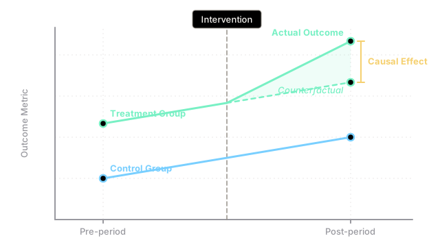
If two cities have always grown at the exact same rate, and then one gets a new ML feature while the other doesn't, any sudden change in their growth rate must be caused by the new feature.
Why Does This Exist?
When you analyze observational data, the biggest fear is unmeasured confounding. If you use Propensity Score Matching to compare users with the same age and income, but you forget to match on "motivation," your estimate of the causal effect is completely wrong.
Difference-in-Differences (DiD) is a quasi-experimental method that solves the unmeasured confounder problem, as long as you have data collected over time. It allows you to estimate causal effects even when the treatment and control groups are fundamentally different, by leveraging the assumption that their trends over time are the same.
This makes it incredibly popular for evaluating policy changes, geo-experiments (e.g., launching a feature in New York but not Boston), and sudden product rollouts where randomized A/B testing is impossible.
Think of It Like This
Think of It Like This
Imagine two runners, Alice and Bob. Alice is inherently faster than Bob; she always finishes a mile exactly 1 minute faster than him. (This 1-minute gap is unmeasured confounding).
One day, Alice drinks a new energy drink before a race, and Bob just drinks water. Alice finishes the mile 3 minutes faster than Bob.
Because we know they usually have a 1-minute gap, we can subtract that baseline difference. The remaining 2-minute improvement must be the causal effect of the energy drink. We didn't need to know why Alice is faster normally (genetics, training, shoes); we only needed to know that the gap is usually stable.
How It Actually Works
Difference-in-Differences requires two groups (Treatment and Control) and two time periods (Pre-Treatment and Post-Treatment).
The Math
We calculate four average outcomes:
- : Treatment group before the intervention.
- : Treatment group after the intervention.
- : Control group before the intervention.
- : Control group after the intervention.
The First Difference (for the Control group) is . This tells us how much the outcome changed naturally due to time (e.g., a seasonal spike in sales). The Second Difference (for the Treatment group) is . This tells us how much the outcome changed due to time plus the treatment.
The causal effect is the Difference in these Differences:
The Parallel Trends Assumption
This math only works if we assume the Parallel Trends Assumption: In the absence of treatment, the difference between the treatment and control groups is constant over time. If the control group goes up by 10%, we assume the treatment group would have gone up by 10% if they hadn't received the treatment. If this assumption fails (e.g., the treatment group was already accelerating faster than the control group before the intervention), DiD will give you the wrong answer.
Code
You don't actually calculate the four averages manually. You run an OLS regression with an interaction term. This allows you to easily add control variables and calculate p-values.
import pandas as pdimport statsmodels.formula.api as smf
# Simulated dataset of daily sales for two cities# city: "NYC" (Treatment) or "Boston" (Control)# time: 0 (Before ML rollout) or 1 (After ML rollout)# treated: 1 (NYC) or 0 (Boston)# post: 1 (After rollout) or 0 (Before rollout)# sales: Daily sales revenue
# We use the standard DiD regression formula:# Outcome = Intercept + beta_1*(treated) + beta_2*(post) + beta_3*(treated * post)
model = smf.ols('sales ~ treated + post + treated:post', data=df).fit()print(model.summary())
# Interpreting the coefficients:# Intercept: Average sales in Boston before the rollout (C_pre)# treated: The baseline difference between NYC and Boston (Unmeasured confounding)# post: The natural change over time (Seasonality)# treated:post: The actual Causal Effect of the ML rollout! (The Difference in Differences)Watch Out For
Failing the Parallel Trends Assumption.
You cannot test this assumption mathematically for the post-treatment period (because it is a counterfactual), but you must visually verify it in the pre-treatment period. Plot the outcome for both groups over time for months before the intervention. If the lines are not parallel before the intervention, you cannot use DiD.
Spillover Effects.
If you roll out a new ML pricing algorithm in New York (Treatment) and keep Boston as Control, what happens if New York customers start telling their friends in Boston about the new prices? If the treatment affects the control group, the difference-in-differences math collapses.
The Quick Version
- Difference-in-Differences estimates causal effects in observational data across time.
- It calculates the natural change over time in a Control group, and subtracts that from the change over time in a Treatment group.
- By subtracting the baseline difference, it automatically controls for unmeasured confounders that are constant over time.
- It relies entirely on the Parallel Trends Assumption: the two groups must have moved in perfect lockstep before the intervention.