Core ML

Long Short-Term Memory

Give the network a separate memory line that gates control instead of overwrite, so relevant information from many steps back can survive untouched until it's needed.

The cell state runs straight across the top as a highway that three gates read and edit — forget multiplies it, input adds to it, output decides how much of it becomes the hidden state

Why Does This Exist?

A vanilla RNN hits a specific wall: its hidden state gets fully recomputed at every step through a $\tanh$ nonlinearity, and the gradient that would teach it to remember something from 50 steps back has to survive 50 multiplications on the way there. In practice it doesn't. Ask a plain RNN to recall the subject of a sentence when it finally reaches the verb, twenty words later, and it usually can't — the information is either overwritten or the gradient carrying "this mattered" has decayed to nothing before training ever sees it.

The fix that shipped in 1997 didn't try to make the existing hidden-state update numerically nicer. It restructured the network around a second piece of state whose entire job is not getting squashed through a nonlinearity every step, and whose contents are edited deliberately rather than overwritten wholesale.

Think of It Like This

A whiteboard with an eraser, a marker, and a window

Picture a running project whiteboard. Most of what's written stays untouched for a long time — it's not rewritten from scratch at every meeting. Three small actions happen instead: someone erases the lines that are no longer relevant (forget), someone adds new notes for what just came up (input), and someone glances at the board to decide what to actually say out loud in this meeting (output) — which is usually a filtered version of what's written, not the whole board.

The whiteboard itself — the cell state — persists unchanged except where one of those three actions deliberately touches it. That's the entire difference from a vanilla RNN, where the whole board gets erased and rewritten every single step whether anything needed to change or not.

How It Actually Works

Three gates, one memory line

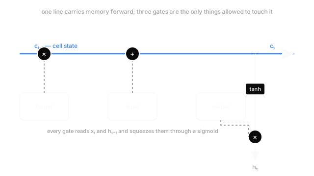
The diagram above shows the cell state $c_{t-1} \to c_t$ running straight across, edited by exactly three gates. Each gate is a small feedforward layer — a sigmoid over $[x_t, h_{t-1}]$ — producing a vector of values between 0 and 1, one per memory dimension, that acts as a per-dimension "how much."

The forget gate decides what to erase:

f_t = \sigma(W_f [x_t, h_{t-1}] + b_f)

A value near 0 in some dimension erases that dimension of the cell state; near 1 keeps it. This gate is multiplicative — it scales the existing memory down, never adds anything.

The input gate decides what to write, working alongside a candidate value $\tilde{c}_t = \tanh(W_c[x_t, h_{t-1}] + b_c)$ :

i_t = \sigma(W_i [x_t, h_{t-1}] + b_i)

The cell state update combines both gates in one line:

c_t = f_t \odot c_{t-1} + i_t \odot \tilde{c}_t

( $\odot$ is elementwise multiplication.) Forget scales down what's already there; input adds a new, gated candidate on top. Nothing here forces a full rewrite — if $f_t \approx 1$ and $i_t \approx 0$ everywhere, $c_t \approx c_{t-1}$ , and the memory survives this step completely untouched.

The output gate decides what the rest of the network actually sees this step:

o_t = \sigma(W_o [x_t, h_{t-1}] + b_o), \qquad h_t = o_t \odot \tanh(c_t)

$h_t$ is the hidden state that feeds the next layer or a prediction — a filtered, squashed view of the cell state, not the cell state itself.

Why this actually fixes the gradient problem

Look at the cell-state update again: $c_t = f_t \odot c_{t-1} + i_t \odot \tilde{c}_t$ . The path from $c_{t-1}$ to $c_t$ is a multiplication by $f_t$ — a learned, per-dimension gate — not a matrix multiply chained through $\tanh$ the way a vanilla RNN's hidden state is. When the network learns $f_t \approx 1$ for a dimension worth preserving, the gradient through that dimension across that step is also close to 1. Chain a hundred steps where $f_t \approx 1$ and the gradient survives a hundred steps, because it was never forced through a saturating nonlinearity along the way. The forget gate isn't just a memory-control knob — it's simultaneously a gradient-control knob, and that's the actual mechanism behind "long" in the name.

Show Me the Code

One LSTM cell step, with the four sub-computations kept visible rather than fused into a single matrix multiply.

1import numpy as np2
3
4def sigmoid(z: np.ndarray) -> np.ndarray:5    return 1.0 / (1.0 + np.exp(-z))6
7
8def lstm_step(9    x_t: np.ndarray, h_prev: np.ndarray, c_prev: np.ndarray, w: dict[str, np.ndarray]10) -> tuple[np.ndarray, np.ndarray]:11    z = np.concatenate([x_t, h_prev])  # combined input, fed to every gate12    f_t = sigmoid(w["f"] @ z)          # forget gate: how much of c_prev survives13    i_t = sigmoid(w["i"] @ z)          # input gate: how much of the candidate to add14    c_tilde = np.tanh(w["c"] @ z)      # candidate memory content15    o_t = sigmoid(w["o"] @ z)          # output gate: how much of c_t becomes h_t16    c_t = f_t * c_prev + i_t * c_tilde17    h_t = o_t * np.tanh(c_t)18    return h_t, c_t19
20
21rng = np.random.default_rng(0)22weights = {k: rng.normal(scale=0.3, size=(4, 6)) for k in ("f", "i", "c", "o")}23h, c = np.zeros(4), np.zeros(4)24h, c = lstm_step(np.array([1.0, 0.0]), h, c, weights)25print(np.round(c, 3))  # -> [ 0.062 -0.02  -0.031  0.056]

The f_t * c_prev term is the one line to remember. Set every entry of f_t to 1 and every entry of i_t to 0, and c_t equals c_prev exactly — untouched memory, by construction.

Watch Out For

Initializing the forget gate to erase by default

With weights initialized near zero, $f_t = \sigma(0) = 0.5$ — the cell state decays by half at every step before the network has learned anything. Some implementations initialize the forget-gate bias to a small positive value (around 1) specifically so training starts closer to "remember by default" rather than "forget by default," which measurably speeds up learning long-range dependencies. Check your framework's default before assuming it's neutral.

Confusing the cell state with the hidden state

$c_t$ and $h_t$ are two different objects — the cell state is the long-lived memory line, the hidden state is what's actually passed to the next layer or used for prediction at this step. A common bug is feeding $c_t$ where $h_t$ was expected (or vice versa) when wiring a custom LSTM by hand. They have the same shape, so nothing crashes; the network just trains worse, quietly, because the output gate's filtering never happens.

The Quick Version

An LSTM adds a separate cell state alongside the hidden state, edited by three sigmoid gates instead of fully overwritten each step.
The forget gate scales existing memory down; the input gate adds a new gated candidate; the output gate filters what the rest of the network sees.
The cell-state update is additive and gate-controlled, not a full nonlinear rewrite — that's what lets gradients survive many steps.
A forget gate near 1 for a dimension means both "keep this" and "the gradient through this dimension survives," which is the actual fix for vanishing gradients.
Cell state and hidden state are different objects with different jobs — don't conflate them.