Propensity Score Methods
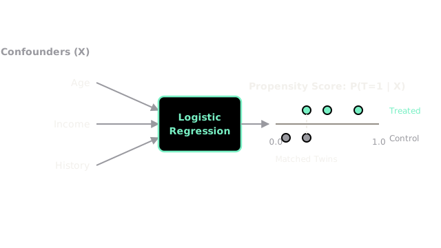
When you can't run an A/B test, you have to mimic one. Propensity scores compress all of a user's confounding traits into a single probability, allowing you to match treated users with identical control users.
Why Does This Exist?
Randomized A/B testing is the gold standard for finding causal effects, but it isn't always possible. You cannot randomly force half your users to smoke cigarettes to see if it causes cancer. You cannot randomly force half your customers to churn to see how it affects your revenue. You are stuck with observational data.
In observational data, the treatment and control groups look totally different. The people who chose to use your new ML feature might be younger, wealthier, and more tech-savvy than the people who didn't. If you just compare their average outcomes, you suffer from massive confounding bias.
Propensity Score Methods exist to artificially reconstruct a randomized experiment out of biased observational data. They do this by finding control users who look exactly like the treated users, and throwing away (or down-weighting) everyone else.
Think of It Like This
Think of It Like This
Imagine you want to know if wearing a smartwatch makes people healthier. If you just look at the data, smartwatch wearers are healthier—but they are also richer and already care more about fitness.
To find the true effect, you find a 30-year-old marathon runner who makes $100k and wears a smartwatch. Then, you search your entire database to find another 30-year-old marathon runner who makes $100k, but who doesn't wear a smartwatch. Because they are practically identical "twins" on every confounding trait, the only difference between them is the watch. By comparing these matched twins, you isolate the causal effect.
How It Actually Works
Finding exact twins in a dataset with 50 features is impossible due to the curse of dimensionality. The Propensity Score Theorem (Rosenbaum and Rubin, 1983) solves this by proving you don't need to match on all 50 features. You only need to match on the probability of receiving the treatment.
1. Calculate the Propensity Score
We train a standard supervised machine learning model (often Logistic Regression or Gradient Boosting).
- Features (X): All the confounding variables (age, income, past behavior).
- Target (Y): Did they receive the treatment? (1 or 0).
The output of this model is the Propensity Score . It is a single number between 0 and 1 that represents how likely this user was to get the treatment, given their traits.
2. Check for Overlap (Common Support)
If a treated user has a score of 0.99, but the highest control user has a score of 0.40, we cannot match them. They are too fundamentally different. We must ensure there is Overlap (Common Support) in the distributions of propensity scores between the two groups. Users at the extreme edges who have no match must be dropped.
3. Estimate the Effect
Once we have the scores, we can estimate the Average Treatment Effect (ATE) in a few ways:
- Propensity Score Matching (PSM): For every treated user, find the control user with the closest propensity score. Calculate the difference in their outcomes.
- Inverse Probability Weighting (IPW): Create a synthetic population where everyone is treated equally by weighting the data. A treated user with a low propensity score of 0.1 is rare, so they get a massive weight (). A control user who looked like they should have been treated (score 0.9) also gets a massive weight ().
Code
Here is a simplified example of Inverse Probability Weighting (IPW) using Logistic Regression to calculate the propensity scores.
import numpy as npimport pandas as pdfrom sklearn.linear_model import LogisticRegressionimport statsmodels.api as sm
np.random.seed(42)N = 10000
# 1. Generate biased observational dataage = np.random.normal(40, 10, N)income = np.random.normal(60000, 20000, N)
# Treatment assignment is highly biased by age and income (Confounders)logit_p = -3 + 0.05 * (age - 40) + 0.00005 * (income - 60000)prob_treatment = 1 / (1 + np.exp(-logit_p))treatment = np.random.binomial(1, prob_treatment)
# True Causal Effect is +500outcome = 1000 + 500 * treatment + 10 * age + 0.05 * income + np.random.normal(0, 100, N)
df = pd.DataFrame({'age': age, 'income': income, 'treatment': treatment, 'outcome': outcome})
# Naive comparison (Biased)naive_ate = df[df['treatment']==1]['outcome'].mean() - df[df['treatment']==0]['outcome'].mean()print(f"Naive ATE: {naive_ate:.2f}") # -> ~ +1100 (Massively overestimates the true effect of +500)
# 2. Calculate Propensity ScoresX = df[['age', 'income']]ps_model = LogisticRegression().fit(X, df['treatment'])df['propensity_score'] = ps_model.predict_proba(X)[:, 1]
# 3. Calculate IPW Weights# Weight for treated: 1 / p# Weight for control: 1 / (1 - p)df['weight'] = np.where(df['treatment'] == 1, 1 / df['propensity_score'], 1 / (1 - df['propensity_score']))
# 4. Estimate Causal Effect using Weighted Least Squares (WLS)X_ipw = sm.add_constant(df['treatment'])ipw_model = sm.WLS(df['outcome'], X_ipw, weights=df['weight']).fit()
print(f"IPW ATE (Causal): {ipw_model.params['treatment']:.2f}")# -> ~ +500 (Recovers the true causal effect!)Watch Out For
Unmeasured Confounders.
Propensity scores only balance the variables you actually put into the model. If there is a massive confounder (like "motivation") that isn't in your database, your matched twins will still be fundamentally different, and your IPW estimate will still be biased. Propensity scores cannot save you from missing data.
Including Colliders in the PS Model.
If you throw every column in your database into the Logistic Regression to calculate the propensity score, you might accidentally include a Collider or a post-treatment Mediator. Doing this actively induces bias. You must construct a Causal Graph first to select only the true confounders for your propensity model.
The Quick Version
- Propensity Score: The probability that a user receives the treatment, based solely on their observed characteristics.
- It compresses a high-dimensional set of confounding variables down to a single number between 0 and 1.
- You can use this score to Match treated and control users who are statistically identical, or use Inverse Probability Weighting (IPW) to balance the dataset.
- It only works if you have actually measured all the important confounders, and if there is overlap (common support) between the two groups.