Core ML

Temporal Convolutional Networks

Stack causal, dilated convolutions instead of a recurrent loop, so a sequence model can be trained with every position processed in parallel rather than one step at a time.

Stacking causal convolutions with doubling dilation lets one output see far back in time using only a few layers, and every position in a layer computes in parallel instead of waiting on the last

Why Does This Exist?

Every recurrent architecture in this band shares one structural constraint: computing $h_t$ requires $h_{t-1}$ to already exist. That's the definition of recurrence, not an implementation detail you can optimize away. Training on a 1,000-step sequence means 1,000 sequential operations that cannot be parallelized across time, however much GPU compute is sitting idle, because step 500 genuinely cannot start before step 499 finishes.

Convolutions don't have that problem. A convolutional layer computes every output position from a local window of the input, and those windows don't depend on each other — position 500's output and position 1's output can be computed simultaneously, on different cores, because neither one waits on the other. The question a temporal convolutional network (TCN) answers is whether that parallelism can be brought to sequence modeling without giving up the two things recurrence was good at: respecting the order of time, and reaching arbitrarily far back into the past.

Think of It Like This

A telescope with adjustable zoom, stacked in layers

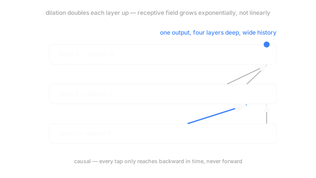
Recall a plain convolution's receptive field: stack enough layers and a single output pixel ends up depending on an ever-wider patch of the original input, one layer's worth of width at a time. A TCN uses the same idea but changes the zoom at each layer instead of the size: the first layer looks at immediate neighbors, the second layer skips outward and looks two steps at a time, the third skips four steps at a time, doubling every layer up.

It's like a telescope whose magnification doubles at each stage — four stages in, you're covering a huge span of history with the same three or four lenses you started with, not by making any single lens bigger, but by spacing the lenses' reach out exponentially.

How It Actually Works

Causal: never look at the future

A TCN's first constraint is causality: the output at position $t$ may only depend on inputs at positions $\leq t$ , never on anything later in the sequence. This is enforced structurally, by padding the input on the left and sliding the convolution kernel so it only ever reaches backward. It's the same requirement autoregressive generation imposes on a recurrent decoder — the future isn't available yet — just enforced through kernel placement instead of through the natural one-step-at-a-time order recurrence gives you for free.

Dilated: reach far back without huge kernels

A plain causal convolution with a kernel of size $k$ only reaches $k$ positions back per layer, so covering a long history the naive way needs either enormous kernels or enormous depth. Dilated convolutions fix this by spacing the kernel's taps out: a dilation of $d$ means the kernel reads every $d$ -th position instead of every consecutive one. Stack layers with dilation doubling at each level — 1, 2, 4, 8, and so on, exactly as the diagram shows — and the receptive field grows exponentially with depth instead of linearly:

\text{receptive field} = 1 + (k - 1) \sum_{i=0}^{L-1} d_i

For $k=2$ and dilations $1, 2, 4, 8$ across four layers, that's $1 + 1 \cdot (1+2+4+8) = 16$ — a history of 16 positions using only four layers and a kernel size of 2 per layer. A vanilla RNN reaches that same history with 16 sequential steps; a TCN reaches it with four layers, each of which processes every position in parallel.

Residual blocks, stacked

In practice, each dilated causal convolution is wrapped in a residual block — the same identity-plus-correction structure from residual connections — which is what makes stacking many dilation levels trainable at all, for the same reasons it makes deep CNNs trainable. Weight normalization and dropout applied per residual block round out the architecture used in the original TCN benchmarks.

What TCNs give up

None of this comes free. A TCN's receptive field, however large, is still fixed — set by the kernel size and dilation schedule at architecture-design time. A recurrent network's hidden state, by contrast, can in principle carry information from arbitrarily far back, however imperfectly, because nothing about the architecture caps how far the recurrence can theoretically reach. For sequences that occasionally need context far beyond whatever receptive field you designed for, a TCN simply doesn't have access to it — you'd need to redesign the dilation schedule and retrain, not just feed a longer sequence in.

Show Me the Code

A causal, dilated 1D convolution over a short sequence, with the causal padding and the dilation spacing both made explicit.

1import numpy as np2
3
4def causal_dilated_conv(x: np.ndarray, kernel: np.ndarray, dilation: int) -> np.ndarray:5    """x: (T,) sequence. kernel: (k,) weights. Output length matches input (causal padding)."""6    k = len(kernel)7    pad = (k - 1) * dilation                          # left-pad only -- never look ahead8    x_padded = np.concatenate([np.zeros(pad), x])9    out = np.zeros_like(x)10    for t in range(len(x)):11        taps = x_padded[t : t + pad + 1 : dilation][-k:]  # every `dilation`-th position back12        out[t] = np.dot(taps, kernel)13    return out14
15
16sequence = np.array([1.0, 2.0, 3.0, 4.0, 5.0, 6.0, 7.0, 8.0])17kernel = np.array([0.5, 0.5])18print(causal_dilated_conv(sequence, kernel, dilation=1))  # -> [0.5 1.5 2.5 3.5 4.5 5.5 6.5 7.5]19print(causal_dilated_conv(sequence, kernel, dilation=2))  # -> [0.5 1.  2.5 3.  4.5 5.  6.5 7. ]

With dilation=1, each output blends a position with its immediate predecessor. With dilation=2, the same two-weight kernel reaches back twice as far per layer, at the same computational cost per output — that's the entire dilation trick.

Watch Out For

Sizing the receptive field smaller than the task needs

The receptive-field formula above is a hard ceiling, not a guideline: a TCN cannot use context from outside it, full stop, however well-trained it is. A common mistake is transplanting a dilation schedule from a paper without recomputing whether it actually covers your sequence's relevant history — a schedule tuned for 500-step audio clips may cover only a fraction of a 5,000-step sensor stream. Compute the receptive field explicitly from your kernel size, dilation schedule, and depth before training, and check it against how far back your task genuinely needs to reach.

Treating parallel training as parallel inference too

Training a TCN is fully parallel across time because the whole input sequence is already known. Autoregressive generation with a TCN isn't automatically parallel in the same way — producing position $t+1$ still needs position $t$ 's output when the model is generating rather than scoring a complete sequence, so naive generation still proceeds one step at a time. The parallelism this page emphasizes is a training-time and full-sequence-scoring advantage; don't assume it eliminates sequential generation cost as well.

The Quick Version

Recurrent networks process a sequence one step at a time, which blocks parallelism across the time dimension during training.
A TCN replaces recurrence with stacked causal, dilated convolutions, so every position in a layer computes independently and in parallel.
Causal padding ensures no position depends on anything later in the sequence.
Dilation doubling per layer grows the receptive field exponentially with depth, instead of linearly with a plain convolution's kernel size.
The receptive field is fixed at design time — unlike a recurrent hidden state, a TCN cannot reach beyond whatever depth and dilation schedule it was built with.