Data Concepts

Feature Scaling

Scaling only matters when the algorithm compares columns to each other. If it only compares a column against a threshold, the numbers can stay as they are.

Unscaled columns stretch the loss into a narrow ravine that descent has to zigzag down, and scaling turns the same loss into near-circular contours one learning rate can cross

Why Does This Exist?

Two columns: annual_income in the tens of thousands, years_experience in single digits. Run K-nearest-neighbours and the distance between two people is, to three decimals, the difference in their incomes. Experience contributes nothing.

Nobody chose that. It fell out of the units.

Here's the rule that replaces the memorised list. Scaling matters exactly when the algorithm computes a distance, a dot product, or a penalty across columns. All three add contributions from different columns into one number, and a sum only means something when its terms are comparable. If the algorithm only compares a column against a threshold, scaling changes nothing.

Think of It Like This

Two judges and one broken score sheet

Two judges rate every act in a contest. One scores 1 to 10. The other read the rules differently and scores 1 to 1000.

You add the scores. The first judge's opinion is now decoration: an act they hate, scored 900 by the second judge, beats an act they love at 10 plus 890.

Put both on a common footing — standard deviations above that judge's own average — and both votes count. You stopped adding centimetres to kilograms.

Now the other half. If the rule were "an act advances when either judge puts it in their own top three", the mismatched scales wouldn't matter — each judge is only compared against themselves.

That second rule is a tree.

How It Actually Works

Apply the rule and the list falls out.

Needs scaling:

KNN and K-means, because both are literally a distance.
SVM with an RBF kernel, where the kernel is a distance and gamma one width for all of it.
PCA, which maximises variance, so the biggest raw variance wins the first component.
Any L1- or L2-penalised linear model, because the penalty sums coefficients across columns, and small units mean a big coefficient to punish.
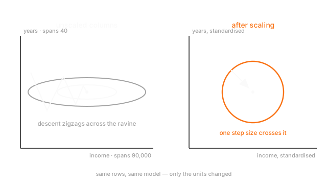
Every neural network trained by gradient descent, because unscaled inputs stretch the loss surface into a thin ravine where one step size can't serve both directions.

Doesn't need scaling: trees, random forests, gradient boosting. A tree asks x > 3; after standardisation it asks x > -0.42, and both send exactly the same rows left and right. Not harmful, just pointless.

The three methods

Standardisation subtracts the mean and divides by the standard deviation:

z = \frac{x - \mu}{\sigma}

$\mu$ is the mean, $\sigma$ the standard deviation. Output has mean 0 and standard deviation 1, unbounded. The default.

Min-max squashes into a fixed interval, usually 0 to 1, as $(x - \min)/(\max - \min)$ . For when something downstream needs bounded input. Both parameters come from two rows, so one extreme value sets max.

Robust scaling subtracts the median and divides by the interquartile range $Q_3 - Q_1$ , the width of the middle half. Both depend on rank, not magnitude, so extreme values barely move them. The answer when outliers are present.

Row scaling is a different thing

Unit-norm scaling divides each row by its own length. Column scaling makes features comparable to each other; row scaling makes records comparable in direction and discards magnitude, which is what cosine similarity wants.

Sparse columns

A sparse matrix stores only its non-zeros. Subtract a mean and every stored zero becomes $-\mu$ , so a 0.1%-full matrix becomes 100% full and stops fitting in memory. Use with_mean=False or MaxAbsScaler.

Worked example

The column [10, 12, 11, 13, 1000]. Four ordinary values, one outlier.

Min-max has min 10 and max 1000, a range of 990: $(12-10)/990 = 0.00202$ , $(11-10)/990 = 0.00101$ , $(13-10)/990 = 0.00303$ , with 10 at 0 and 1000 at 1.

Robust scaling uses the median, 12, and the IQR: sorted, the values are 10, 11, 12, 13, 1000, so $Q_1 = 11$ , $Q_3 = 13$ , IQR 2. That gives $-1.0$ , $-0.5$ , $0$ , $0.5$ , and $(1000-12)/2 = 494$ .

All three are affine, so the shape never changes — only where the numbers land. Min-max handed the top of its range to one row, squeezing the rest into its first 0.3%. Robust scaling gave the ordinary values a window of 1.5 and left the outlier at 494, visible and available for a decision. Standardisation suffers too: its 395 standard deviation came mostly from the outlier.

Show Me the Code

1import numpy as np2
3x: np.ndarray = np.array([10.0, 12.0, 11.0, 13.0, 1000.0])  # four ordinary values, one outlier4
5def min_max(a: np.ndarray) -> np.ndarray:6    return (a - a.min()) / (a.max() - a.min())7
8def standardise(a: np.ndarray) -> np.ndarray:9    return (a - a.mean()) / a.std()          # a.std() here is 395.4, mostly the outlier10
11def robust_scale(a: np.ndarray) -> np.ndarray:12    q1, q3 = np.percentile(a, [25, 75])      # -> 11.0 13.0, so the IQR is 2.013    return (a - np.median(a)) / (q3 - q1)14
15print(np.round(min_max(x), 5).tolist())      # -> [0.0, 0.00202, 0.00101, 0.00303, 1.0]16print(np.round(standardise(x), 3).tolist())  # -> [-0.504, -0.499, -0.501, -0.496, 2.0]17print(np.round(robust_scale(x), 2).tolist()) # -> [-1.0, 0.0, -0.5, 0.5, 494.0]

Read the first and last lines together: min-max leaves the ordinary values in a window of about 0.003, robust scaling in one of 1.5.

Watch Out For

Fitting the scaler on everything, or refitting it at serving time

scaler.fit_transform(X) followed by train_test_split fits the mean and standard deviation on rows you're about to hold out, so the test set was standardised using knowledge of itself. The validation number improves and production doesn't. That's data leakage.

The stranger version is at serving. Refit on each incoming batch and the same customer scores differently depending on who else arrived: alone they look average, alongside a whale they're an outlier. Nothing errors, and it isn't reproducible in principle.

Fit once, on training rows, and persist the parameters with the model artefact.

Scaling columns that shouldn't be, or a target you forget to invert

StandardScaler on the whole frame hits your one-hot columns too. A binary indicator becomes something like -0.31 and 3.2 — annoying for a linear model's interpretability, and it destroys the sparsity you were counting on. Select numeric columns by name with a ColumnTransformer.

Scaling the target is separate. Often right for a network, and it means your model no longer predicts prices, it predicts standardised prices. Skip the inverse and your metric is in units nobody recognises and your predictions are out by orders of magnitude.

The Quick Version

Scaling matters when the algorithm computes a distance, a dot product, or a penalty across columns. Otherwise it doesn't.
Needed for KNN, K-means, RBF SVM, PCA, regularised linear models, and gradient-descent-trained networks.
Irrelevant for trees and boosting: x > 3 and its scaled equivalent split identically.
Standardisation is the default, min-max when you need bounded output, robust scaling when outliers are present.
Min-max takes both parameters from two rows, so one extreme value flattens the rest into a sliver.
Unit-norm row scaling is different: records compared by direction, not columns aligned.
Never subtract a mean from a sparse matrix; use with_mean=False or MaxAbs.
Fit on training rows, persist the parameters, never refit at serving.