Data Concepts

Preference Data Collection

Asking which of two answers is better is far more reliable than asking someone to score one. Every aligned model is built on that switch from rating to ranking.

Two annotators using different parts of a five-point scale disagree on the same answer's rating while agreeing perfectly on which of two answers is better, which is why preference data is collected as comparisons

Why Does This Exist?

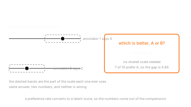
Ask ten people to rate a chatbot response out of five and you get numbers that don't mean the same thing. One person's 4 is another's 2. Some never use the extremes, some never use the middle, and every rater's scale drifts over an afternoon.

Ask the same ten people which of two responses is better and agreement jumps, because the question no longer depends on where anyone anchors a scale. It's a comparison, and humans are far better at comparisons than at absolute judgements.

That switch is the foundation under every aligned model. You can't write a loss function for "be helpful", and you can't reliably collect a number for it either. What you can collect is a pile of comparisons, fit a model that scores responses consistently with them, and optimise against that.

The whole operation is a data-collection problem wearing an alignment hat, which is why it belongs here rather than with the training algorithms.

Think of It Like This

Judging cheese without a scale

Ask a hundred people to score a cheese out of ten and the answers are mush. Some are generous, some are harsh, some anchor on the last cheese they ate, and one person has decided 7 is the highest any cheese can be.

Hand them two cheeses and ask which they prefer, and the data gets sharp. Nobody needs a shared idea of what 7 means. Each person only has to compare two things in front of them, which is what tasting is.

Then the useful part: enough pairwise verdicts across enough pairs reconstructs a full ranking, and you can put a number on each cheese afterwards — derived from the comparisons rather than asked for directly. Those numbers are comparable, because they came from one consistent fit rather than a hundred private scales.

How It Actually Works

What one record looks like

A prompt, two or more candidate responses, and a verdict: which was preferred. Optionally a strength ("much better" against "slightly better"), a tie option, and a written rationale — which costs more and is worth it, because rationales are how you debug the guidelines.

Where the candidates come from matters more than people expect. Sample them from the model you intend to improve, at a realistic temperature, because preferences over responses your model would never produce don't tell you how to improve it. Preference data goes stale as the model changes, which is why collection is continuous rather than a one-off dataset.

Turning comparisons into scores

The standard bridge is the Bradley-Terry model: assume each response has a latent quality score, and the chance one is preferred is a sigmoid of the difference.

P(A \succ B) = \sigma(r_A - r_B)

Read it plainly: $r_A$ and $r_B$ are the two latent scores, and $\sigma$ squashes their difference into a probability. Invert it and a preference rate becomes a score gap. If annotators prefer A seven times in ten, the gap is $\ln(0.7/0.3) = 0.85$ . A near-tie at 55% is a gap of 0.20; a clear 95% win is 2.94.

That inversion is what a reward model learns to predict, and it's why comparisons are enough — you never needed the absolute numbers.

The agreement ceiling, and it's low

Human-human agreement on open-ended preference tasks typically lands between 60% and 75%. That's much lower than a classification task, and it is a hard ceiling: a reward model cannot be more consistent than the preferences it was fitted to, so measure it before drawing conclusions from small differences.

The practical implication is uncomfortable. If your annotators agree 68% of the time, a reward model at 70% accuracy is close to the achievable limit, and chasing 80% means fixing the guidelines rather than the model.

The biases that get baked in

Preference data encodes whatever your annotators reward, including things nobody intended.

Length. Annotators prefer longer answers, substantially, well past the point of usefulness. Uncorrected, this is the single largest artefact in preference datasets, and it's why aligned models became verbose.

Confidence and formatting. A confident, well-structured wrong answer beats a hedged correct one. Bullet points and headings score well on their own.

Position. Whichever response is shown first has an advantage, so randomise the order and log which position each was in.

Sycophancy. Responses agreeing with the prompt's premise get preferred, which teaches the model to agree.

Every one of these becomes a target the model optimises, and that's reward hacking: the model finds the artefact rather than the intent. Control for length explicitly, ablate formatting, and check whether your reward model can be fooled by padding before you trust it.

AI feedback

Using a strong model as the judge is now standard, because it's orders of magnitude cheaper and more consistent than humans. It's also a labelling function with all that implies: correlated errors, its own position and length biases, and a preference for text that resembles its own output.

The workable pattern is a hybrid — AI judgements for volume, a human-labelled subset to calibrate against, and a measured agreement rate between the two that you monitor rather than assume.

Worked example

Ten annotators compare response A against response B. Seven prefer A.

Under Bradley-Terry that 0.7 preference rate is a reward gap of $\ln(0.7/0.3) = 0.8473$ . Push it back through the sigmoid and you recover 0.7 exactly, which is the round trip a reward model is trained to reproduce.

Now the sensitivity. A 55/45 split is a gap of 0.2007 — small, and within sampling noise on ten comparisons. A 95/5 split is 2.9444. So the same scale spans an order of magnitude between "barely distinguishable" and "clearly better", and with only ten comparisons per pair you cannot tell 0.55 from 0.60.

That's the argument for volume over precision: many pairs compared a few times each beats few pairs compared many times, because the reward model fits across pairs.

Show Me the Code

1import numpy as np2
3wins_a: int = 74comparisons: int = 105
6def reward_gap(p_a_wins: float) -> float:7    """Bradley-Terry inverted: a preference rate becomes a latent score difference."""8    return float(np.log(p_a_wins / (1 - p_a_wins)))9
10def preference_rate(gap: float) -> float:11    return float(1 / (1 + np.exp(-gap)))12
13p: float = wins_a / comparisons14print(p, round(reward_gap(p), 4))                # -> 0.7 0.847315print(round(preference_rate(reward_gap(p)), 4))  # -> 0.7      the round trip16print(round(reward_gap(0.55), 4))                # -> 0.2007   a near-tie is a small gap17print(round(reward_gap(0.95), 4))                # -> 2.9444   a clear win is a large one

Note what a 50/50 split would do: $\ln(1) = 0$ , so a tie carries no information about the gap at all. Ties need collecting and then handling deliberately, not dropping.

Watch Out For

Length going uncontrolled

You collect 50,000 comparisons, fit a reward model, optimise against it, and the model's answers get noticeably longer. Reviewers say quality improved. Users say it waffles.

The mechanism is plain: annotators prefer longer responses, so length correlates with the preference label, so the reward model learns length as a feature. Optimising against it optimises length, and that's the largest single artefact in preference data.

Two things make it hard to spot. Longer answers genuinely are better sometimes, so the correlation isn't spurious, just over-weighted. And your reward model's accuracy on held-out comparisons stays high, because the held-out comparisons have the same bias.

Measure it: correlate response length with the preference label across your dataset, and check whether your reward model prefers the same answer with filler appended. If it does, you have a length model. Then control for it — match candidate lengths within a pair where you can, or include length as an explicit term you can regress out.

Trusting an AI judge you never calibrated

An AI judge gives you 500,000 comparisons for the price of 500 human ones, so the human collection stops.

Now every bias of that judge is your reward signal. It prefers its own phrasing, so a model optimised against it converges toward the judge's style rather than toward quality. It has position and length biases of its own, usually stronger than a human's. And its errors are correlated, so unlike human noise they don't average out with volume — a hundred thousand judgements from one model is closer to one opinion repeated than to a hundred thousand opinions.

You also lose the ability to notice. Without a human-labelled subset, there's no measurement that would tell you the judge drifted after a version upgrade.

Keep a rolling human-labelled calibration set, report judge-human agreement as a tracked metric, and randomise candidate order in every judge prompt. If agreement drops below your human-human rate, the judge is the weaker annotator and volume won't fix it.

The Quick Version

Absolute ratings don't survive contact with multiple annotators. Comparisons do, because they don't depend on a shared scale.
One record is a prompt, two or more candidates, and a verdict. Sample candidates from the model you're improving, or the data won't apply to it.
Bradley-Terry turns a preference rate into a score gap: 70% is 0.85, 55% is 0.20, 95% is 2.94, and a tie is 0.
Human-human agreement on open-ended preferences runs 60 to 75%, and that's a ceiling on any reward model.
Length is the biggest artefact in preference data, and optimising against it is why aligned models got verbose.
Confidence, formatting, position and sycophancy all get rewarded. Randomise order and ablate formatting.
Reward hacking is the model finding the artefact instead of the intent. Test whether padding fools your reward model.
AI judges are cheap and correlated, so volume doesn't average out their errors. Keep a human calibration set and track agreement.
Many pairs judged a few times beats few pairs judged many times.