SQL for Feature Extraction
A GROUP BY hands you one row per key. A window function hands you one row per row, and correct feature extraction almost always needs that second shape.
Why Does This Exist?
Most features get computed in the warehouse, not in Python. Whatever the SQL got wrong arrives as a column with a sensible name and no null in it.
This isn't a SQL tutorial. Assume joins, GROUP BY, CASE WHEN. What's here is the slice that decides whether features are correct: window functions, temporal joins, sessionisation, as-of correctness.
GROUP BY customer_id collapses a million events into one row per customer. Your model needs a value per prediction, and a customer gets scored many times. A GROUP BY gives one row per key. A window function gives one row per row, and feature extraction needs the second.
Think of It Like This
The running balance beside each line
A bank statement carries two numbers on every line: what that transaction was worth, and the running balance after it.
The total at the bottom is a GROUP BY: one number for the whole account. Fine for a tax return, useless for "could they have afforded £400 on 14 March", because it includes April and everything after.
The running balance answers that. It sits on the line, built from that line plus everything above it. Nothing below. One extra column, and its whole meaning comes from where the window stops.
How It Actually Works
One clause does the work: OVER (PARTITION BY user_id ORDER BY event_ts). PARTITION BY says which rows can see each other, ORDER BY says in what order, and the row count out matches the row count in.
The functions that earn their keep
ROW_NUMBER()picks one record per key: number rows by descending timestamp and keep number 1.RANK()lets ties share a number, so it can return two.LAG(x)gives deltas.event_ts - LAG(event_ts) OVER (...)is the gap since the previous event, the most reusable lag feature there is.LEADlooks forward, so on a feature table it's a bug.- Framed aggregates.
AVG(amount) OVER (... ROWS BETWEEN 6 PRECEDING AND CURRENT ROW)is a 7-row rolling mean;RANGE BETWEEN INTERVAL '30 days' PRECEDING AND CURRENT ROWis a real 30-day window. Seven rows might span a day or a year. SUM(...) OVER (...)with no frame expands from the start of the partition to here: lifetime counts, cumulative spend.
Where the frame ends is the whole game
ORDER BY inside OVER with no frame written gives RANGE BETWEEN UNBOUNDED PRECEDING AND CURRENT ROW, usually right. Drop the ORDER BY too and the frame becomes the whole partition, future included. CURRENT ROW against UNBOUNDED FOLLOWING is the difference between a feature and a leak, in two words nobody reviews.
The as-of join
Labels and facts run on different clocks, and you need the newest fact known strictly before a row's prediction stamp. Union the streams, order by timestamp, and carry the fact forward with LAST_VALUE(...) OVER (... ROWS UNBOUNDED PRECEDING) — or use ASOF JOIN. The condition is a strict inequality: equal timestamps mean the fact landed the instant you predicted, which in practice means after.
Sessionisation, the two-step
event_ts - LAG(event_ts) OVER (...) > INTERVAL '30 minutes' is a flag meaning "this starts a session". Then SUM(flag::int) OVER (... ROWS UNBOUNDED PRECEDING) — the running total of those flags is the session id. It only increments, and only where you wanted a break. The same trick does streaks and restarts.
Two things that quietly lie
LEFT JOIN plus COUNT(*) returns one for an empty child table: the outer join manufactured a row of nulls, and COUNT(*) counts rows. Use COUNT(child.id). And WHERE runs before windows compute, so filter a window's output with QUALIFY or a subquery.
Worked example
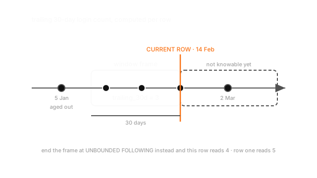
One user, five logins: 5 Jan, 20 Jan, 1 Feb, 14 Feb, 2 Mar. Count each row's logins in the trailing 30 days, inclusive.
Row one has nothing before it: 1. Row two catches row one: 2. Row three catches both: 3. Row four's window opens 15 Jan and drops row one, so still 3. Row five's opens 31 Jan and drops two: 3. The column reads 1, 2, 3, 3, 3.
Swap CURRENT ROW for UNBOUNDED FOLLOWING and it reads 5, 5, 5, 4, 3. Row one now claims five logins by 5 January. One had happened.
Code
SQL this time, because the bug is a SQL bug.
-- One user, five logins: 5 Jan, 20 Jan, 1 Feb, 14 Feb, 2 Mar 2026.WITH logins(user_id, event_ts) AS ( VALUES (1, DATE '2026-01-05'), (1, DATE '2026-01-20'), (1, DATE '2026-02-01'), (1, DATE '2026-02-14'), (1, DATE '2026-03-02'))SELECT event_ts, COUNT(*) OVER (PARTITION BY user_id ORDER BY event_ts RANGE BETWEEN INTERVAL '30 days' PRECEDING AND CURRENT ROW) AS trailing_30d, COUNT(*) OVER (PARTITION BY user_id ORDER BY event_ts RANGE BETWEEN INTERVAL '30 days' PRECEDING AND UNBOUNDED FOLLOWING) AS leaky_30dFROM loginsORDER BY event_ts;-- trailing_30d -> 1, 2, 3, 3, 3 frame ends at this row-- leaky_30d -> 5, 5, 5, 4, 3 frame runs off the end of the table-- Row one is the whole page: one login existed on 5 Jan, and column two says five.Two words changed. Both columns are non-null integers that look like counts, and only one can be computed in production.
Watch Out For
A frame you didn't write, ordered by a column you didn't check
The ORDER BY inside OVER decides what "before" means. Order by updated_at when you meant event_ts, and "everything preceding this row" means preceding in a sequence unrelated to time.
No error. The column populates, the distribution looks plausible, and the model finds it. An omitted ORDER BY is worse: the frame becomes the whole partition, so every row carries an aggregate over that customer's future.
Write the frame out even when the default is right, and pick one event clock. Then score a temporal holdout against a random split. See data leakage.
A point-in-time join written as an equality on a date
JOIN dim_customer d ON d.customer_id = f.customer_id AND d.snapshot_date = f.event_date. Tidy, indexable, wrong in two directions.
With no snapshot on that exact date the row drops or arrives null, so the join silently loses rows. With one present you get the version stored under that date, possibly corrected weeks later.
The worse case is structural: a dimension updated in place has no history, so it can't answer "what did we know then" at all. You need validity ranges or an append-only log you can replay, and that decision predates the feature. Data versioning has the shape that works.
The Quick Version
- A
GROUP BYreturns one row per key; a window function returns one per row, which is what a feature table needs. OVER (PARTITION BY ... ORDER BY ...)is the whole idea. The rest is which function and which frame.ROW_NUMBERpicks the latest record per key,LAGgives deltas, framed aggregates roll, unframedSUMexpands.ROWS BETWEEN 6 PRECEDINGcounts rows,RANGE ... INTERVAL '30 days' PRECEDINGcounts days, and noORDER BYgives the whole partition.CURRENT ROWagainstUNBOUNDED FOLLOWINGturned1, 2, 3, 3, 3into5, 5, 5, 4, 3, silently.- An as-of join matches on a strict inequality. Equality on a date isn't one.
- Sessionisation is
LAGfor a gap flag, then a runningSUMof flags as the session id. LEFT JOINwithCOUNT(*)returns one for an empty child; useCOUNT(child.id).WHEREfilters before windows compute,QUALIFYafter.