Data Concepts

Synthetic Data Generation

A generator only samples from a distribution it learned, so synthetic data adds coverage and never adds information. Train on it, then test on real data.

Refit a generator on its own output and the distribution narrows every round, so the tails you built it for are the first thing to disappear

Why Does This Exist?

You need 50,000 labelled examples of a failure mode that happens four times a year. You need to hand a dataset to a partner who is not allowed to see your customers. You need crash footage without crashing anything.

In all three cases you generate the data. This is no longer a curiosity — synthetic instruction data, synthetic preference data and simulated environments are load-bearing parts of how current models get built.

One sentence covers the whole trade, and it's worth holding onto because it predicts every success and every failure below. A generator can only produce samples from a distribution it learned, so synthetic data adds coverage and never adds information.

Coverage is genuinely valuable: more examples in thin regions, balanced classes, rare combinations you can enumerate rather than wait for. But nothing in the output tells you anything the source data didn't already imply. If your real data never contained a failure at −20°C, no generator will invent one correctly.

Think of It Like This

A photocopy of a photocopy

Copy a page. It's fine — you can read it, and a casual glance won't tell you it's a copy.

Copy the copy. Still readable, slightly softer. Do it forty times and you have a grey rectangle with the ghost of a headline in it. Nothing dramatic happened at any single step, and every generation was a faithful reproduction of the one in front of it.

What went first? Not the headline. The faint pencil note in the margin, the hairline rule, the thin serifs. Detail at the edges of what the machine could resolve.

That's what happens to a distribution's tails when a generator is trained on generated data. The common cases survive a long time. The rare ones — the reason you wanted more data — go in the first few rounds.

How It Actually Works

The methods, and what each one gets wrong

Rules and simulation. Write the generator by hand: a physics engine, a traffic simulator, a templated document. Total control, exact labels, unlimited volume. The failure has a name — the reality gap. A model trained only in simulation meets real sensor noise, real lighting, real dirt on the lens, and falls over. Domain randomisation is the standard mitigation: vary textures, lighting and physics parameters far more wildly than reality, so reality becomes one unremarkable sample inside the training distribution.

VAEs learn a smooth latent space you can interpolate through and sample from, at the cost of blurry samples, because the objective rewards covering the data rather than committing to sharp output.

GANs invert that trade: sharp samples, unstable training, and mode collapse — the generator finds a handful of outputs that reliably fool the discriminator and stops covering the rest of the distribution. Your samples look excellent and represent a fraction of your data.

Diffusion models are the current default for images and audio. They cover modes well and cost a lot to sample from, since generation is an iterative denoising process rather than one forward pass.

LLM generation for text and tabular rows is now the most common route by volume. Worth knowing: an LLM's output distribution is far narrower than its apparent fluency suggests. Ask for 1,000 customer complaints and you'll get remarkable uniformity of structure, sentiment and length unless you work hard at the prompting.

Two risks that need naming

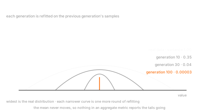
Model collapse. Train a generator on data that includes its own output, repeatedly, and the distribution narrows every round. The mechanism is unglamorous: a sample variance estimated from finite data runs low, and refitting on those samples bakes the shortfall in permanently. Do it again and you lose the same fraction again. It compounds, it's monotone, and the tails go first.

This matters at two scales: your own pipeline if you're bootstrapping generations, and the open web as a training corpus now that a growing share of it is generated.

Privacy is not automatic. "It's synthetic" is not a privacy argument. A generator can memorise and reproduce a training record more or less verbatim, especially a rare one — and rare records are exactly the re-identifiable ones. If privacy is the reason you're generating, you need differential privacy in the training of the generator, or a membership-inference test on its output, or both. Data privacy and governance covers what those actually buy you.

Evaluation, where projects go wrong

One rule, and it's absolute. Never evaluate on synthetic data. Train on synthetic, test on real — often written TSTR — and report per slice, because synthetic data usually helps the head of the distribution and hurts the tail.

For tabular data, check the joint distribution and not only the marginals. It's easy to match every column's histogram while destroying the correlation structure, and a model trained on that learns relationships that don't exist. A quick check: train a classifier to distinguish real rows from synthetic ones. If it gets 99% accuracy, your synthetic data is trivially distinguishable and the relationships are probably wrong too.

Worked example

Take a real distribution with variance 1.0. Draw 10 samples, fit a Gaussian to them, then draw 10 samples from the fit and repeat.

A sample variance computed on $n$ draws underestimates the true variance by a factor of $(n-1)/n$ on average, so each generation keeps 90% of the previous variance at $n = 10$ . That compounds:

\text{variance after } k \text{ generations} = \left(\frac{n-1}{n}\right)^k

At generation 10 the variance is 0.349. At generation 30 it's 0.042. At generation 100 it's 0.0000266, which is a spike at the mean.

Sample size is the whole lever. At $n = 1000$ , generation 30 still holds 0.970 of the variance. So collapse is not a mystical property of generated data — it's what happens when each round is fitted on too few samples, and it is arithmetic you can compute in advance.

Show Me the Code

1import numpy as np2
3n: int = 10             # samples drawn per generation4sigma2: float = 1.0     # the variance of the real data we start from5
6def variance_after(generations: int, rows: int = n) -> float:7    """Each refit keeps (rows-1)/rows of the variance, because a sample variance runs low."""8    return sigma2 * ((rows - 1) / rows) ** generations9
10print(round(variance_after(0), 5))              # -> 1.011print(round(variance_after(10), 5))             # -> 0.3486812print(round(variance_after(30), 5))             # -> 0.0423913print(round(variance_after(100), 8))            # -> 2.656e-05   a spike at the mean14print(round(variance_after(30, rows=1000), 5))  # -> 0.97043     sample size is the lever

The last line is the useful one: same recursion, 1,000 samples per round instead of 10, and thirty generations cost you 3% instead of 96%.

Watch Out For

Reporting a score measured on synthetic data

You generate 200,000 rows, split them into train and test, fit a model, and report 0.94.

That number measures how consistently your generator agrees with itself. Both halves came from the same learned distribution, so the model only had to reproduce the generator's regularities — including the ones that aren't in the real world. It's a closed loop with a metric attached.

The version that gets past review is subtler: real training data topped up with synthetic rows, then a test split taken after mixing. Now synthetic rows are in the test set, and rows generated from a real training row sit beside their parent across the split, which is duplicate leakage with a generator in front of it.

Keep a real, untouched test set from the start. Generate only into the training fold. Report train-synthetic-test-real, and report it per slice so you can see the tail separately from the head.

Recursive generation with no fresh real data

Round one is real data plus generated data, and it helps. So round two trains the generator on that mixture, and round three on the next one, because each round looked fine.

Variance decays every round, monotonically, in exactly the way the arithmetic above predicts. And it doesn't announce itself: mean behaviour is preserved, aggregate metrics look stable, and standard summary statistics barely move at first. The tails go first, which means the rare classes you built the pipeline to cover are the first casualties.

Three defences. Anchor every generation to the original real data rather than the previous generation. Track a distributional statistic across rounds — a variance, a tail quantile, a distinct-value count — and treat monotone shrinkage as a stop condition. And keep provenance on every row, so "which generation is this from" is answerable a year later. Dataset documentation is where that lives.

The Quick Version

A generator samples from a distribution it learned. Synthetic data adds coverage, never information.
It earns its place for rare classes, unshareable data, dangerous or expensive scenarios, and where labelling is the bottleneck.
Simulation gives control and a reality gap; domain randomisation is the standard fix.
VAEs are smooth and blurry. GANs are sharp and mode-collapse. Diffusion covers well and costs to sample. LLM output is narrower than it looks.
Model collapse is arithmetic: at 10 samples per round each generation keeps 90% of the variance, so generation 30 holds 0.042. At 1,000 samples it holds 0.970.
The tails disappear first, and the tails are why you generated.
"It's synthetic" is not a privacy claim. Generators memorise rare records, which are the re-identifiable ones.
Never evaluate on synthetic data. Train synthetic, test real, report per slice.
For tabular data check the joint distribution, not just each column's histogram.