Flow-Based Models (Normalizing Flows)
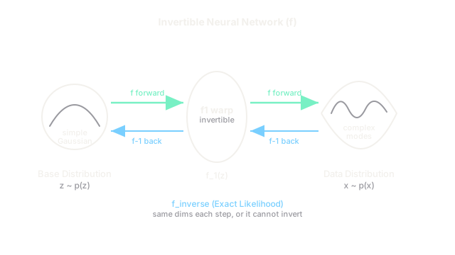
Flow-based models use a sequence of mathematically reversible funhouse mirrors to perfectly morph a simple block of clay (noise) into a complex statue (an image), allowing you to exactly calculate the probability of any given statue existing.
Why Does This Exist?
In generative AI, we generally want to do two things: generate new data that looks real, and calculate exactly how real a specific piece of data is (its likelihood or probability).
Generative Adversarial Networks (GANs) generate beautiful images but have no mathematical way to tell you the probability of an image. Variational Autoencoders (VAEs) can estimate the probability, but it's only a lower bound (an approximation), so their images tend to be blurry. Diffusion models calculate probability by simulating an SDE over hundreds of steps, which is incredibly slow.
Flow-based models (Normalizing Flows) were designed to be the mathematical holy grail: a model that can generate high-quality data and calculate the exact, perfect probability of that data in a single pass. They achieve this by strictly limiting the neural network to only use mathematical operations that can be perfectly reversed.
Think of It Like This
The Origami Master
Imagine a flat, square piece of paper. This represents a simple, boring probability distribution (like a standard Gaussian bell curve). We understand the paper perfectly; we know the exact coordinates of every point on it.
A Normalizing Flow is an origami master who folds the paper into a complex paper crane (a complex data distribution, like human faces).
However, the master must obey one strict rule: No cutting, no tearing, and no gluing. Every single fold must be perfectly reversible. Because of this rule, if you hand the master a finished paper crane, they can perfectly unfold it back into the flat square. Because the folding process is perfectly reversible, we can calculate the exact probability of the paper crane existing just by looking at the original flat square of paper.
How It Actually Works
Flow-based models rely on a fundamental theorem from probability calculus called the Change of Variables Formula.
1. The Change of Variables Formula
If you have a simple probability distribution (like noise) and you pass it through a mathematical function to get complex data, how do you find the probability of ? Calculus tells us that . The scary-looking term on the right is the determinant of the Jacobian matrix. It simply measures how much the function stretches or squishes the space. If the function stretches the space by a factor of 2, the probability density drops by half.
2. Invertible Neural Networks
To use this formula, the neural network must meet two extremely strict criteria:
- It must be perfectly invertible: must guarantee . If a neural network loses information (e.g., downsampling from 64x64 to 32x32), it cannot be inverted. Flow models cannot use standard bottlenecks.
- The Jacobian determinant must be easy to calculate: For a standard neural network with millions of parameters, calculating this determinant takes time, which would take years to compute for a single image.
Researchers solved this by inventing specialized neural network layers (like Coupling Layers in models like RealNVP and GLOW). These layers use a clever masking trick where half the data is passed through unchanged, and the other half is modified based on the first half. This guarantees perfect invertibility and makes the Jacobian determinant mathematically trivial to compute in real-time.
3. Normalizing the Flow
You stack dozens of these reversible layers together. You start with complex data , pass it backward through the inverted network , and force the output to look like a standard normal Gaussian (a bell curve). By doing this, you are "normalizing" the complex data into a simple shape. To generate a new image, you just sample random noise from the bell curve and pass it forward through to get an image.
Code
This code demonstrates a highly simplified Affine Coupling Layer, the backbone of invertible neural networks like RealNVP. Notice how the inverse function perfectly unwinds the forward function.
import torchimport torch.nn as nn
class AffineCouplingLayer(nn.Module): def __init__(self, channels): super().__init__() # A standard, NON-invertible neural network used to calculate scale (s) and translation (t) # It only operates on half the channels. self.net = nn.Sequential( nn.Linear(channels // 2, 64), nn.ReLU(), nn.Linear(64, channels) # Outputs both s and t )
def forward(self, x): # 1. Split the data exactly in half x1, x2 = x.chunk(2, dim=-1) # 2. Calculate scale and translation using only the FIRST half s_and_t = self.net(x1) s, t = s_and_t.chunk(2, dim=-1) # 3. Modify the SECOND half, leave the first half alone # We use torch.exp(s) to ensure the scale is strictly positive y1 = x1 y2 = x2 * torch.exp(s) + t # 4. Recombine return torch.cat([y1, y2], dim=-1)
def inverse(self, y): # Perfect invertibility! y1, y2 = y.chunk(2, dim=-1) # We can calculate the exact same s and t because y1 == x1 s_and_t = self.net(y1) s, t = s_and_t.chunk(2, dim=-1) # Reverse the math x1 = y1 x2 = (y2 - t) * torch.exp(-s) return torch.cat([x1, x2], dim=-1)Watch Out For
The Dimensionality Curse
Because flow-based models must be perfectly invertible, the input and output must have the exact same number of dimensions. You cannot compress a 1024x1024 image into a 64x64 latent space like a VAE or Stable Diffusion does. If your image has 3 million pixels, your noise vector must have exactly 3 million pixels, and every single layer of the network must process 3 million pixels. This makes Normalizing Flows incredibly memory-intensive and very difficult to scale to high-resolution images compared to Diffusion or GANs.
The Quick Version
- Normalizing Flows are generative models that can calculate the exact mathematical probability of the data they generate.
- To achieve this, the entire neural network must be built out of perfectly invertible, mathematically reversible operations.
- They rely on the Change of Variables formula to stretch and squish a simple Gaussian bell curve perfectly into a complex data distribution.
- While mathematically elegant and useful for scientific data, their inability to compress data (due to the strict invertibility requirement) makes them too computationally expensive to compete with Diffusion models for high-resolution image generation.