Fisher Information

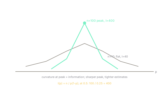
Fisher information measures how sharply data pin down a parameter. Sharp likelihood peaks mean tight estimates; flat ones mean the data barely speak.

Ten flips give a flat likelihood with information 40 while a hundred flips sharpen the peak to information 400

Why Does This Exist?

Two experiments can share an estimate and differ tenfold in trustworthiness: 6 of 10 heads versus 600 of 1000 both say $\\hat p = 0.6$ , but the second pins $p$ down while the first barely constrains it. The estimate alone cannot tell them apart.

Fisher information $I(\\theta) = \\mathrm{Var}(\\nabla_\\theta \\log p(X;\\theta)) = -\\mathbb{E}[\\nabla^2_\\theta \\log p]$ does. It is expected curvature: sharp peaks carry information, flat ones do not. It sets the Cramer-Rao floor, drives Wald intervals, and parameterizes Jeffreys priors. It assumes maximum likelihood estimation and feeds the Cramer-Rao bound.

The one idea you need first

The score $s(\\theta) = \\nabla_\\theta \\log p(x;\\theta)$ points uphill on log-likelihood with mean zero. Its variance measures how strongly data tug the parameter. Curvature averages that tug.

Think of It Like This

A valley in fog

You stand in a valley in fog and feel the slope underfoot. A sharp V tells your position within a step; a wide flat bowl leaves you guessing across meters. Fisher information is the valley's curvature at your feet.

Observed information is the ground you actually feel today; expected information averages over all weather. Where it stops: curvature is local. A sharp local valley inside a multimodal landscape still misleads globally.

How It Actually Works

Under regularity (support free of $\\theta$ , differentiation under the integral), $I_n(\\theta) = n\\,i_1(\\theta)$ adds per observation. For Bernoulli( $p$ ): $i_1(p) = 1/(p(1-p))$ , so $I_n = n/(p(1-p))$ . Wald intervals use $\\hat\\theta \\pm z\\,I(\\hat\\theta)^{-1/2}$ . The information matrix generalizes to vectors; natural gradients precondition steps by it.

Worked example

Hundred flips at $p = 0.5$ : $I = 100/0.25 = 400$ . Standard-error floor $1/\\sqrt{400} = 0.05$ . At $p = 0.6$ : $I = 100/0.24 \\approx 416.7$ , floor $\\approx 0.049$ . Ten flips at $0.5$ give $I = 40$ , floor $\\approx 0.158$ : same estimate scale, triple the wobble. Information turns "more data" into a number.

Code

1import numpy as np2
3n, p = 100, 0.54info = n / (p * (1 - p))  # Bernoulli Fisher information5print(round(float(info), 1))  # -> 400.06print(round(float(1 / np.sqrt(info)), 3))  # -> 0.05

Information 400 gives a 0.05 precision floor. The code is the definition, evaluated where it matters.

Watch Out For

Quoting expected information under misspecification

$I(\\theta)$ averages under the assumed model. Under misspecification the true sampling wobble follows the sandwich $H^{-1}VH^{-1}$ , not $I^{-1}$ . Model-based intervals then run narrow and overconfident.

Use observed information or sandwich errors when the model is a working approximation. If residuals look structured, distrust $I^{-1}$ .

Ignoring the boundary

Near $p = 0$ or $1$ , Bernoulli information $1/(p(1-p))$ explodes and regularity frays: the MLE piles at the boundary and asymptotics break. Wald intervals can spill outside $[0,1]$ .

Reparameterize (logit), use exact or profile intervals, or penalize. If estimates sit on the edge, the curvature number is fiction.

The Quick Version

Fisher information is expected log-likelihood curvature: sharp peaks, tight estimates.
Bernoulli: $I_n = n/(p(1-p))$ ; 100 flips at 0.5 give 400 and a 0.05 floor.
Information adds per observation under regularity.
It drives Cramer-Rao floors, Wald intervals, and natural gradients.
Misspecification needs sandwich errors, not $I^{-1}$ .
Boundary parameters break the asymptotics; reparameterize or go exact.