Interpolation Methods

Interpolation fills in the missing gaps between known data points by estimating intermediate values using adjacent neighbours.

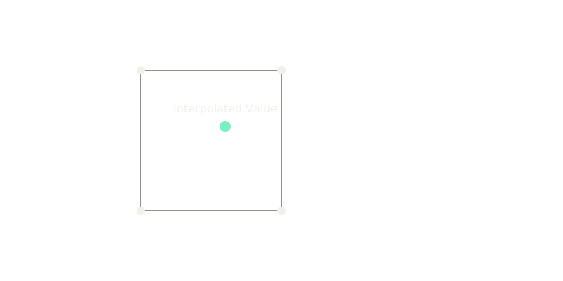
Estimating an unknown value from surrounding known data points.

Why Does This Exist?

When resizing images, transforming coordinates, or upsampling discrete data grids, we often need to look up a value at a continuous floating-point coordinate that falls between our known integer grid points. Interpolation methods calculate a plausible value for these continuous coordinates.

Think of It Like This

If you know the temperature at the top of a mountain and at the base, you can guess the temperature halfway up. Interpolation is simply standardising the mathematical rules for how you blend those known values based on how close you are to each of them.

How It Actually Works

The two most common 2D spatial interpolation methods are bilinear and bicubic:

Bilinear Interpolation: Performs linear interpolation in one direction (e.g., along the x-axis) and then applies another linear interpolation on those results in the perpendicular direction (e.g., along the y-axis). It takes the 4 nearest neighbors into account. The resulting surface is a quadratic equation, not a true plane.
Bicubic Interpolation: Goes a step further by fitting a cubic polynomial surface using the nearest 16 pixels ( $4 \times 4$ grid). This method preserves edges better and reduces the blocky artifacts seen in simpler methods, resulting in a smoother image when upscaling.
Weighting: Both methods ultimately compute the new pixel as a weighted sum of the surrounding known pixels, where the weights are determined by the fractional distance to the continuous coordinate.

Code

1def bilinear_interpolate(x: float, y: float, values: list[list[float]]) -> float:2    # Interpolates a point in a unit square with corner values3    # values: [[top_left, top_right], [bottom_left, bottom_right]]4    5    top = values[0][0] * (1 - x) + values[0][1] * x6    bottom = values[1][0] * (1 - x) + values[1][1] * x7    8    return top * (1 - y) + bottom * y9
10grid = [[10.0, 20.0], 11        [30.0, 40.0]]12# Point at exactly the center (0.5, 0.5)13print(bilinear_interpolate(0.5, 0.5, grid))14# -> 25.0

Watch Out For

Aliasing: Interpolation methods don't invent new high-frequency detail when upsampling. Bicubic might look smoother than nearest-neighbor, but it can also introduce ringing artifacts or overshoot values slightly beyond the original range.

The Quick Version

Interpolation estimates unknown values between discrete data points.
Bilinear interpolation uses a $2 \times 2$ neighbourhood to compute a weighted average.
Bicubic interpolation uses a $4 \times 4$ neighbourhood for smoother, sharper results.
These methods are essential for image resizing and spatial transformations in vision models.