Math

Matrix Multiplication

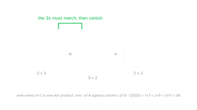
Every entry of the answer is one dot product: a row from the left meeting a column from the right, which is why the inner dimensions have to agree.

Two matrices can only be multiplied when the inner dimensions match, and that shared dimension disappears from the answer: a two-by-three times a three-by-two gives a two-by-two

Why Does This Exist?

A dense layer in a neural network is a matrix multiplication. Not built on one, not similar to one — that is what the layer is, plus a bias add and a nonlinearity. Attention is four of them. A transformer block is a stack of them. When you buy a GPU, what you are really buying is silicon that does this one operation faster than anything else can.

So the practical stakes are unusual for a piece of maths this small. Two things follow from it, and both are the reason to read the whole page rather than just the formula.

First, the shape rule is where most of your errors will come from, because it is the rule that decides whether your layers connect. Second, and less widely understood: the cost of a matmul is usually not the arithmetic. Naive multiplication of two $n \times n$ matrices takes on the order of $n^3$ operations, and that is the number everyone quotes — but on modern hardware the arithmetic often finishes waiting for memory. Knowing which regime you are in is the difference between an optimisation that helps and one that does nothing.

Think of It Like This

A recipe table meeting a price list

You have three recipes, each needing some amount of flour, sugar and butter. That is a table with 3 rows and 3 columns.

Separately you have a price list: what flour, sugar and butter each cost, at two different shops. That is a table with 3 rows — one per ingredient — and 2 columns, one per shop.

Multiply them and you get the cost of every recipe at every shop: 3 rows by 2 columns. Each single answer came from walking down one recipe and one shop's prices together, multiplying amount by price, and totalling.

Notice what had to line up. The recipe table's columns were ingredients, and the price list's rows were ingredients too. That shared meaning is the inner dimension, and it is why the shapes must match — you cannot pair a recipe's amounts against a list of prices for different ingredients. Notice also that ingredients do not appear in the answer at all. They were consumed by the summing.

How It Actually Works

If $A$ has shape $m \times k$ and $B$ has shape $k \times n$ , the product $C = AB$ has shape $m \times n$ , and each entry is the dot product of a row of $A$ with a column of $B$ :

C_{ij} = \sum_{p=1}^{k} A_{ip} B_{pj}

In plain words: to fill in row $i$ , column $j$ of the answer, walk along row $i$ of the left matrix and down column $j$ of the right matrix together, multiplying pairs and adding them up.

The shape rule falls straight out of that. The walk pairs one element of $A$ 's row with one element of $B$ 's column, so those must be the same length. Written as shapes:

(m \times \mathbf{k}) \cdot (\mathbf{k} \times n) \rightarrow (m \times n)

The inner $k$ appears twice, must agree, and is gone from the result. Two useful habits come from this. Reading a chain like $(32 \times 768)(768 \times 3072)(3072 \times 768)$ , you can check it composes by confirming each adjacent pair matches — and you can read off the final shape, $(32 \times 768)$ , without computing anything.

It does not commute, and that is not a technicality

$AB$ and $BA$ are different operations, and often only one of them is even legal. With $A$ at $2 \times 3$ and $B$ at $3 \times 2$ , both happen to be legal — but $AB$ is $2 \times 2$ while $BA$ is $3 \times 3$ . Different shapes, different contents, different meaning.

The dangerous case is when the two orderings produce the same shape, which happens whenever both matrices are square. Then swapping them raises no error and returns a plausible array. In neural network terms, $XW$ (a batch of rows transformed by weights) and $WX$ are genuinely different claims about what your data means, and only one matches your layer's definition.

The cost, and why flops are the wrong thing to count

The operation count is easy: $m \times n$ output entries, each needing $k$ multiplications and $k$ additions, so roughly $2mnk$ floating-point operations. For square $n \times n$ matrices that is $2n^3$ — the cubic scaling everyone knows.

But count the memory traffic too. You have to read $A$ and $B$ and write $C$ : about $3n^2$ numbers moved. The ratio of arithmetic to memory traffic is:

\frac{2n^3}{3n^2} = \frac{2n}{3}

In plain words: bigger matrices do more arithmetic per number fetched from memory. That ratio is called arithmetic intensity, and it decides your bottleneck. Large square matmuls have plenty of arithmetic per byte and can saturate the compute units — those are the ones that hit advertised GPU throughput. Thin or small matmuls do not, so they finish waiting on memory bandwidth and run at a fraction of peak no matter how fast the chip's arithmetic is.

This is the practical reason batching works. Multiplying one $1 \times 768$ input by a $768 \times 3072$ weight matrix is bandwidth-bound: you read the entire weight matrix to do very little arithmetic. Stack 32 inputs into a $32 \times 768$ batch and you read the same weights once but do 32 times the arithmetic. The weights were going to be fetched either way.

Worked example

A = \begin{bmatrix} 1 & 2 & 3 \\ 4 & 5 & 6 \end{bmatrix}, \qquad B = \begin{bmatrix} 7 & 8 \\ 9 & 10 \\ 11 & 12 \end{bmatrix}

Shapes are $2 \times 3$ and $3 \times 2$ , so the inner dimensions are both 3 and the answer is $2 \times 2$ .

Four entries, four dot products. Row 1 of $A$ against column 1 of $B$ : $1 \times 7 + 2 \times 9 + 3 \times 11 = 7 + 18 + 33 = 58$ . Row 1 against column 2: $1 \times 8 + 2 \times 10 + 3 \times 12 = 8 + 20 + 36 = 64$ . Row 2 against column 1: $4 \times 7 + 5 \times 9 + 6 \times 11 = 28 + 45 + 66 = 139$ . Row 2 against column 2: $4 \times 8 + 5 \times 10 + 6 \times 12 = 32 + 50 + 72 = 154$ .

AB = \begin{bmatrix} 58 & 64 \\ 139 & 154 \end{bmatrix}

Reversing the order is legal here and gives a $3 \times 3$ matrix instead — a completely different object, which is the non-commutativity point made concrete.

Show Me the Code

1import numpy as np2
3A = np.array([[1, 2, 3], [4, 5, 6]])          # shape (2, 3)4B = np.array([[7, 8], [9, 10], [11, 12]])     # shape (3, 2)5
6print((A @ B).shape, (A @ B).tolist())   # -> (2, 2) [[58, 64], [139, 154]]7print((B @ A).shape)                     # -> (3, 3)  legal, and a different thing8
9# Every entry is one dot product — row i of A against column j of B.10print(A[0] @ B[:, 0])                    # -> 5811
12# The classic silent error: * is elementwise, @ is matmul. Both can succeed.13S = np.array([[1, 2], [3, 4]])14print((S * S).tolist())                  # -> [[1, 4], [9, 16]]    elementwise15print((S @ S).tolist())                  # -> [[7, 10], [15, 22]]  matmul

The last pair is worth internalising. On square matrices * and @ both return the right shape and neither warns you, so a typo there is a wrong answer rather than a crash.

Watch Out For

Using the elementwise operator where you meant matmul

In NumPy and PyTorch, * multiplies elementwise and @ multiplies matrices. On square inputs both are legal and both return the same shape, so swapping them produces a numerically different result with no error and no warning.

It is easy to write, because * is what multiplication looks like in every other context. And it is hard to spot afterwards, because a model built on elementwise products still trains — it just represents something much weaker than the linear layer you designed, and you go looking for capacity problems instead.

The one place this reliably bites is porting maths from a paper. Papers write $XW$ with no operator, and the mental translation to code is where the substitution happens. When you are transcribing a formula, check every product against its shapes: if the inner dimensions differ, it must be @; if they are identical, decide deliberately rather than by habit.

Getting the batch axis wrong in a batched matmul

@ on tensors of rank 3 or higher multiplies the last two axes and broadcasts everything in front of them as batch. So $(8, 32, 64) \mathbin{@} (8, 64, 16)$ does eight independent $32 \times 64$ by $64 \times 16$ multiplications and returns $(8, 32, 16)$ . That is usually what you want.

The failure comes from a batch axis in the wrong position. If your data arrives as $(32, 8, 64)$ — sequence-first rather than batch-first — the operation still runs. It just treats 32 as the batch count and multiplies the wrong pairs together, quietly mixing information across examples that should never have met.

This is the bug behind a model that performs well in training and collapses at inference with a batch size of one, because a stray axis of length 1 broadcasts differently from an axis of length 32. Print the shape before and after every batched matmul while you are wiring it up, and assert the batch axis is where you think it is.

The Quick Version

Each entry of the product is one dot product: a row of the left against a column of the right.
$(m \times k)(k \times n) \rightarrow (m \times n)$ . The inner dimension must match and then disappears.
Read a chain of shapes to check it composes and to get the output shape without computing anything.
$AB \neq BA$ . On square matrices the swap is legal and silently wrong.
Cost is about $2mnk$ operations against roughly $3n^2$ numbers moved, so arithmetic intensity grows with size.
Small or thin matmuls are memory-bandwidth-bound, not compute-bound. That is why batching pays.
* is elementwise, @ is matmul, and on square inputs both succeed.
Batched matmul acts on the last two axes and broadcasts the rest. Verify where your batch axis sits.