Objective Functions and Constraints

The objective says what "best" means and the constraints say what is allowed. Every training run minimises one subject to the other.

Minimising x squared with x forced above 3 lands on the fence at exactly 3, because the unconstrained best at zero is forbidden

Why Does This Exist?

"The loss went down" is not the same as "the model is acceptable". A classifier can reach 99% accuracy while assigning probabilities that do not sum to one, a recommender can maximise clicks while showing the same five items, a controller can minimise energy while violating safety limits. The objective function scores how good an answer is; constraints fence off which answers are allowed. Optimisation is the first subject to the second.

Formally: minimise $f(x)$ subject to $x \in C$ , where $C$ is the feasible set. Everything else is technique for handling the fence. Penalties fold violations into the objective ( $f(x) + \lambda \cdot \text{violation}$ ). Projection steps back inside after each update. Lagrange multipliers, covered in Lagrange multipliers and duality, price the constraints exactly. The catalog of $f$ 's themselves lives in common loss functions; this page is about the split between goal and fence.

The one idea you need first

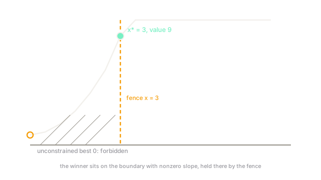
An unconstrained minimum is where the slope vanishes and curvature points up. Add a fence and the winner may sit on the boundary instead, where the slope is not zero at all: it pushes into the fence and the fence pushes back. That balance of two pushes is the entire content of constrained optimality.

Think of It Like This

The cheapest flat inside the school zone

You want the cheapest flat in the city (the objective: minimise rent). But your kid's school requires living inside the school zone (the constraint: location within the boundary).

Without the zone you would take the cheapest flat anywhere, maybe far outside town. With it, the answer is the cheapest flat on or inside the boundary, very often sitting exactly on the borderline street. The unconstrained optimum is irrelevant; it is not for sale to you.

Penalties are the "fine per mile outside the zone" version: you may technically look anywhere, but every mile out costs extra. Make the fine huge and the answer converges to the fenced one. That is exactly how penalty methods approximate hard constraints.

How It Actually Works

Three ways to handle the fence:

Projection: step downhill, then map back into $C$ . Cheap when $C$ is simple (a box, a ball, the probability simplex). Projected gradient descent is this loop.
Penalties: minimise $f(x) + \lambda \cdot v(x)$ where $v$ measures violation. Simple and unconstrained, but the answer only satisfies the fence approximately unless $\lambda$ grows without bound.
Lagrange / KKT: introduce a price $\lambda_i \ge 0$ per constraint and solve the stationarity system. Exact, and the prices diagnose which constraints bite.

Constraints come as equalities ( $h(x) = 0$ : probabilities sum to one) or inequalities ( $g(x) \le 0$ : weights stay small). An inequality that holds with room to spare is inactive and can be ignored locally; one sitting at equality is active and shapes the answer.

Worked example

Minimise $f(x) = x^2$ subject to $x \ge 3$ . Unconstrained, the answer is $x = 0$ with value 0. But 0 violates the fence. The objective grows as $|x|$ grows, so the best allowed point hugs the fence as tightly as possible:

x^\star = 3, \quad f(x^\star) = 9

Note the slope at the answer: $f'(3) = 6 \ne 0$ . The minimum sits on the boundary with nonzero slope, held there by the constraint. Any method that hunts "slope equals zero" without checking the fence walks straight past it to the forbidden 0.

Code

The point is the check: project each gradient step back into the feasible set and watch the iterates stick to the boundary.

1def projected_descent(start: float, lr: float, steps: int) -> float:2    x = start3    for _ in range(steps):4        x = x - lr * 2 * x  # downhill on x squared5        if x < 3.0:6            x = 3.0  # project back into x above 37    return x8
9
10print(projected_descent(10.0, 0.1, 50))  # -> 3.0

Starting at 10, the iterates fall until they hit the fence at 3.0, and every later step tries to leave and gets projected back. Remove the projection line and the same loop converges to 0.0: the unconstrained answer to a different problem.

Watch Out For

Optimising the loss while silently leaving the feasible set

A soft penalty with a small weight lets the model trade constraint violations for loss improvements: probabilities that sum to 1.2, "sparse" masks that are dense, budgets that are overspent. If a constraint is a requirement rather than a preference, verify feasibility on the final answer directly instead of assuming the penalty handled it.

Calling a regulariser a constraint

Adding $\lambda \lVert w \rVert^2$ to the loss is not the constraint $\lVert w \rVert \le c$ . The penalty version lets the norm float wherever the trade-off lands; the constrained version pins it. They coincide only for a matched $\lambda$ -to- $c$ mapping you almost never know in advance. Name which one you implemented before claiming its guarantees.

The Quick Version

The objective scores answers; constraints fence off the allowed ones in the feasible set.
Minima can sit on the boundary with nonzero slope, so slope-equals-zero is not the whole test.
Projection, penalties and Lagrange multipliers are the three ways to handle the fence.
Inactive constraints can be ignored locally; active ones shape the answer.
A penalty is not a constraint: verify feasibility on the final answer when it matters.