Sampling Distributions

One sample gives one average. Imagine every possible sample: the averages pile into their own bell, far narrower than the data itself.

Flat die faces on the left become a tight bell of sample means on the right, with standard error 0.28 and only 0.04 of means past 4

Why Does This Exist?

A sample mean is a single draw from a hidden distribution: the distribution of what the mean would be across every sample you could have taken. Without that distribution, 3.6 from 36 rolls means nothing: lucky high roll, or loaded die? With it, the same number becomes evidence with a calibrated strength. Confidence intervals, p-values, and power calculations are all downstream of this one object.

The sampling distribution is also the intuition pump behind the central limit theorem: whatever the data's shape, the means pile into a bell. And its width, the standard error, sets every error bar you have seen in confidence intervals. The data summaries underneath are descriptive statistics.

The one idea you need first

A statistic varies from sample to sample: redraw the data and the mean moves. The sampling distribution is the probability distribution of that movement. Its center is typically the parameter being estimated, and its spread shrinks as samples grow. Everything here is that spread, its size, and its shape.

Think of It Like This

Weighing rice bag after bag

A mill fills nominal one-kilo bags with a sloppy machine: individual bags range widely. Weigh one bag and you learn little. Weigh the average of 36 bags and the number barely moves from filling to filling, because over and under fill cancel.

The bag weights are the population: wide and flat. The 36-bag averages are the sampling distribution: narrow and bell-shaped. Same machine, different object, and confusing them means either panicking over one light bag or trusting one heavy average. The standard error is the scale on the second weighing: it reports how far averages wander, not how far bags do.

The analogy stops at shape. Bag weights here are flat, and averages still bell up. That shape-forgetting is the central limit at work, and it needs enough bags: tiny samples inherit the population's shape instead.

How It Actually Works

For independent draws with population mean $\mu$ and standard deviation $\sigma$ , the sample mean $\bar{X}_n$ over $n$ draws has:

E[\bar{X}_n] = \mu, \qquad \text{SE}(\bar{X}_n) = \frac{\sigma}{\sqrt{n}}

In plain words: averaging preserves the center and divides the spread by $\sqrt{n}$ . The standard error is that divided spread: the standard deviation of the mean, not of the data. Quadruple the sample to halve the error bars; no other lever exists for independent data.

Shape comes free with size. As $n$ grows, the sampling distribution of the mean approaches a normal bell whatever the population looked like, which is the central limit theorem. With $n = 36$ the bell is already close, so normal arithmetic answers questions like the worked probability below.

Worked example

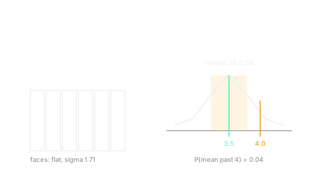
Fair die rolls: $\mu = 3.5$ and $\sigma^2 = 35/12 \approx 2.917$ , so $\sigma \approx 1.708$ .

Average $n = 36$ rolls. The means center on $3.5$ with standard error $1.708 / 6 \approx 0.285$ , six times tighter than single rolls. How surprising is a mean above $4$ ? Standardize: $z = (4 - 3.5) / 0.285 \approx 1.76$ , and the normal tail past $1.76$ is about $0.04$ . So roughly one set of 36 in twenty-five averages above 4 with a fair die. A mean of $4.5$ would sit $3.5$ standard errors out, chance about $0.0002$ : that is the neighborhood where loaded dice get accused.

Code

Twenty thousand simulated sets of 36 rolls, recovering the theoretical center and spread with no formulas.

1import random2
3rng = random.Random(0)4n = 365means = [sum(rng.randint(1, 6) for _ in range(n)) / n for _ in range(20000)]6center = sum(means) / len(means)7spread = (sum((m - center) ** 2 for m in means) / len(means)) ** 0.58print(round(center, 3))  # -> 3.4979print(round(spread, 3))  # -> 0.285

The simulation prints 3.497 and 0.285 against theory 3.5 and 0.285. Flat faces in, tight bell out: the code watches the sampling distribution form.

Watch Out For

Plotting the standard deviation where the standard error belongs

Error bars showing data spread ( $\sigma$ ) when the claim is about the mean ( $\sigma/\sqrt{n}$ ) exaggerate uncertainty by $\sqrt{n}$ , a factor of 6 at $n = 36$ . Readers conclude nothing is significant when the means are actually nailed down. Label every bar as SD or SE, and match the bar to the claim: data claims take SD, mean claims take SE.

Trusting the bell at tiny n on skewed data

The normal approximation earns its keep near $n = 30$ for tame data, but heavy skew or outliers delay it: means of a handful of lognormal draws stay visibly lopsided. Check with a quick simulation like the one above before quoting normal tails, or the 0.04 you report belongs to a bell your means never joined.

The Quick Version

The sampling distribution is the distribution of a statistic across every possible sample.
Means center on the population mean with standard error sigma over root n.
Die means over 36 rolls cluster with spread 0.28, and topping 4 happens about 4 percent of the time.
The bell shape arrives with size regardless of the data's shape, which is the central limit theorem.
Error bars on means use the standard error; the standard deviation describes single draws.