Model Monitoring

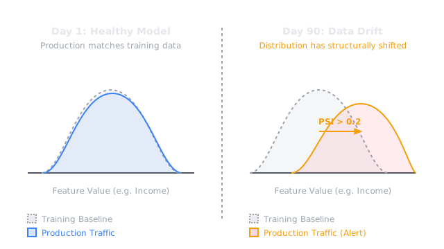
Model monitoring tracks the health of deployed ML models by measuring prediction quality, data drift, and system performance — alerting when the real world has diverged from the training distribution enough to degrade value.

Why Does This Exist?

A deployed model degrades silently. Unlike software, which either works or crashes with an error, an ML model continues returning responses while its predictions quietly become less useful. The world changes — user behavior shifts, economic conditions evolve, new products launch, fraud patterns mutate — and the model trained on yesterday's data serves tomorrow's distribution.

Model monitoring creates the observable feedback loop that software monitoring provides for traditional systems: measure continuously, alert on anomalies, respond before customers notice.

Think of It Like This

A weather station with automated alerts

A weather station measures temperature, pressure, and humidity continuously. It doesn't wait for a hurricane to notice something has changed — it detects the pressure drop that precedes the storm and alerts meteorologists with enough time to respond. Model monitoring works the same way: it measures leading indicators of performance degradation (feature distributions, prediction distributions) and alerts before customers notice degraded service.

How It Actually Works

What to monitor

1. Input feature drift: Are the features arriving at inference time still distributed like the training data?

Statistical tests:

Population Stability Index (PSI): $\text{PSI} = \sum_i (Q_i - P_i) \ln(Q_i / P_i)$ where $P$ = training distribution, $Q$ = current distribution. PSI < 0.1 = negligible; 0.1–0.2 = moderate; > 0.2 = significant drift.
Kolmogorov-Smirnov (KS) test: Non-parametric test comparing CDFs. Reports a p-value.
Jensen-Shannon divergence: Symmetric version of KL divergence, bounded in [0, 1].

2. Output distribution shift: Is the distribution of model predictions changing? A fraud model that was predicting fraud 2% of the time and now predicts 15% either found a real epidemic or has broken.

3. Model performance metrics: Ground-truth performance (accuracy, AUC) — the most direct measure of degradation, but labels arrive with a delay. For a loan default model, you wait months to know if a loan actually defaults.

4. Proxy metrics: Business KPIs that correlate with model quality: click-through rate, conversion rate, support ticket volume. Use these when ground truth labels are delayed.

5. System metrics: Latency, throughput, error rate, memory usage, GPU utilization. Infrastructure health ≠ model quality, but infrastructure failures manifest as bad predictions.

Monitoring cadence

Data volume	Recommended approach
Low traffic	Batch reports (daily/weekly)
Medium traffic	Rolling window statistics (hourly)
High traffic	Streaming monitoring (real-time PSI)

Code

1import pandas as pd2import numpy as np3from evidently import ColumnMapping4from evidently.report import Report5from evidently.metric_preset import DataDriftPreset, DataQualityPreset, TargetDriftPreset6
7# ── Simulate reference (training) and current (production) data ───────────────8np.random.seed(42)9n_ref, n_curr = 5000, 100010
11reference_data = pd.DataFrame({12    "age":               np.random.normal(35, 10, n_ref).clip(18, 80),13    "income":            np.random.exponential(50000, n_ref),14    "days_since_login":  np.random.exponential(7, n_ref),15    "country":           np.random.choice(["US", "UK", "DE", "FR"], n_ref, p=[0.5, 0.2, 0.2, 0.1]),16    "label":             np.random.binomial(1, 0.05, n_ref),17    "prediction":        np.random.beta(1, 19, n_ref),  # model output18})19
20# Simulate drift: income distribution shifts, country mix changes21current_data = pd.DataFrame({22    "age":               np.random.normal(38, 12, n_curr).clip(18, 80),   # slight shift23    "income":            np.random.exponential(40000, n_curr),             # significant shift24    "days_since_login":  np.random.exponential(7, n_curr),                 # stable25    "country":           np.random.choice(["US", "UK", "DE", "FR"], n_curr, p=[0.3, 0.3, 0.3, 0.1]),26    "label":             np.random.binomial(1, 0.08, n_curr),             # label shift27    "prediction":        np.random.beta(1.5, 17, n_curr),                 # output shift28})29
30# ── Configure and run an Evidently report ─────────────────────────────────────31column_mapping = ColumnMapping(32    target="label",33    prediction="prediction",34    numerical_features=["age", "income", "days_since_login"],35    categorical_features=["country"],36)37
38report = Report(metrics=[39    DataDriftPreset(),40    DataQualityPreset(),41    TargetDriftPreset(),42])43
44report.run(45    reference_data=reference_data,46    current_data=current_data,47    column_mapping=column_mapping,48)49
50# Save HTML report51report.save_html("monitoring_report.html")52
53# Programmatic result access54result = report.as_dict()55dataset_drift = result["metrics"][0]["result"]["dataset_drift"]56drift_share = result["metrics"][0]["result"]["share_of_drifted_columns"]57print(f"Dataset drift detected: {dataset_drift}")58print(f"Share of drifted columns: {drift_share:.1%}")

1# ── Manual PSI computation ────────────────────────────────────────────────────2def compute_psi(reference, current, bins=10):3    """Compute Population Stability Index for a numerical feature."""4    # Create bins from reference distribution5    min_val = min(reference.min(), current.min())6    max_val = max(reference.max(), current.max())7    breakpoints = np.linspace(min_val, max_val, bins + 1)8    9    ref_pct = np.histogram(reference, bins=breakpoints)[0] / len(reference) + 1e-610    curr_pct = np.histogram(current, bins=breakpoints)[0] / len(current) + 1e-611    12    psi = np.sum((curr_pct - ref_pct) * np.log(curr_pct / ref_pct))13    return psi14
15psi = compute_psi(reference_data["income"], current_data["income"])16level = "negligible" if psi < 0.1 else "moderate" if psi < 0.2 else "significant"17print(f"Income PSI: {psi:.3f} → {level} drift")

Watch Out For

Monitoring infrastructure but not model quality

A 200 OK response with 5ms latency says nothing about whether the model's predictions are useful. Always monitor at least one model-quality signal — prediction distribution, a proxy business metric, or actual label performance when labels are available. Infrastructure health and model health are orthogonal.

Alert fatigue from over-sensitive thresholds

Setting drift thresholds too low means constant alerts for normal statistical variation. Teams begin ignoring the monitoring dashboard — the worst outcome. Calibrate thresholds by measuring drift during known-good periods (not just applying rule-of-thumb PSI > 0.1). Use rolling baselines that adapt to gradual seasonal shifts rather than a fixed training-data snapshot.

The Quick Version

Model monitoring detects when a deployed model's environment has diverged from its training distribution.
Monitor: input feature drift (PSI, KS test), output distribution shift, model performance (with labels or proxies), and system metrics.
PSI > 0.2 on a key feature is the standard threshold for investigation.
Use proxy business metrics (click-through rate, conversion) when ground-truth labels are delayed.
Calibrate alert thresholds from known-good periods, not arbitrary rules — avoid alert fatigue.