Language Models

Why Does This Exist?

In the early days of natural language processing, researchers attempted to codify language using strict, handwritten grammar rules. They built massive dictionaries and complex syntax trees, hoping to program computers to understand human language by explicitly telling them how it worked. This approach failed because natural language is inherently ambiguous, fluid, and constantly evolving. People break grammar rules routinely, invent new words, and rely heavily on context that rigid rules simply cannot capture.

The shift to language modeling changed everything by reframing language from a problem of rules to a problem of probabilities. A language model exists to calculate how likely a given sequence of words is to occur. When you speak to a voice assistant, it might hear something that sounds like "recognize speech" or "wreck a nice beach." Without a language model, both might seem plausible based on acoustics alone. But a language model knows that the sequence "recognize speech" is statistically far more likely to occur in typical conversation than "wreck a nice beach," allowing the system to output the correct transcription.

Fundamentally, language models exist to assign a probability to a sequence of words, which intrinsically gives them the ability to generate text. By understanding which words typically follow other words, these models can complete sentences, translate text more fluently, and serve as the backbone for modern conversational AI. They are the engine that allows machines to move past strict dictionaries and instead grasp the statistical fabric of human communication.

Think of It Like This

How It Actually Works

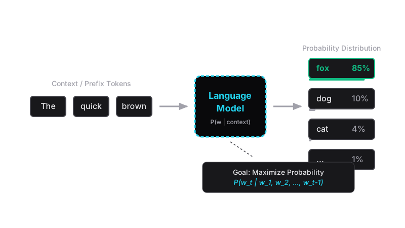
At its mathematical core, a language model is a function that takes a sequence of words (often called tokens) and calculates a probability distribution over the entire vocabulary for the next word.

1. The Chain Rule of Probability

To figure out the probability of an entire sentence like "The cat sat", we can break it down using the chain rule of probability. The probability of the sequence $P(\text{The}, \text{cat}, \text{sat})$ is calculated as the probability of the first word, multiplied by the probability of the second word given the first, multiplied by the probability of the third word given the first two:

$P(\text{The}, \text{cat}, \text{sat}) = P(\text{The}) \times P(\text{cat} \mid \text{The}) \times P(\text{sat} \mid \text{The}, \text{cat})$

While mathematically elegant, computing the exact probability of a word given a very long preceding context (say, a whole paragraph) quickly becomes impossible if you are just counting occurrences in a dataset. You will inevitably encounter sequences that never appeared in your training data, which would give a probability of zero, ruining the calculation.

2. The Markov Assumption and N-grams

To solve the impossibility of infinitely long contexts, classical language models make a simplifying assumption known as the Markov property: we assume that the probability of the next word only depends on a fixed window of previous words, not the entire history.

This leads to the concept of N-gram models. In a bigram model (where $N=2$), the model only looks at the immediately preceding word. The previous equation simplifies dramatically:

$P(\text{The}, \text{cat}, \text{sat}) \approx P(\text{The}) \times P(\text{cat} \mid \text{The}) \times P(\text{sat} \mid \text{cat})$

A trigram model looks at the previous two words, and so on. By restricting the context window, we can simply count how many times "cat" follows "The" in our corpus and divide it by the total occurrences of "The" to estimate the probability. This counting method formed the backbone of NLP for decades.

3. Neural Language Models

While N-gram models are fast, they suffer from data sparsity (many possible combinations never appear in the training data) and lack of semantic understanding (they don't know that "dog" and "cat" are similar words).

Neural language models replaced the simple counting mechanism with neural networks. Instead of looking at exact word matches, they convert words into dense mathematical vectors called embeddings. These embeddings map words into a continuous space where similar words are located closer together. When the model tries to predict the next word, it passes these vectors through layers of a neural network (like an RNN, LSTM, or Transformer), which can synthesize information from a much longer context window than an N-gram model ever could.

The output layer of this neural network produces a set of raw scores—called logits—for every word in the vocabulary.

4. Softmax and Sampling

The final step turns those raw scores into proper probabilities using a softmax function. The softmax squeezes all the scores into a range between 0 and 1, ensuring they all add up to 100%. The model then samples from this distribution. It might pick the word with the highest probability (greedy decoding), or it might introduce some randomness (temperature sampling) to pick a highly probable word that isn't necessarily the top choice, making the generated text more diverse and natural.

Code

This snippet demonstrates a simple character-level bigram frequency count, which is the foundational concept behind classical language modeling.

1from collections import defaultdict2
3def train_bigram_model(text: str) -> dict:4    """Train a simple character-level bigram model."""5    counts = defaultdict(lambda: defaultdict(int))6    7    # Count occurrences of char pairs8    for i in range(len(text) - 1):9        current_char = text[i]10        next_char = text[i+1]11        counts[current_char][next_char] += 112        13    # Convert counts to probabilities14    probabilities = {}15    for char, next_chars in counts.items():16        total_occurrences = sum(next_chars.values())17        probabilities[char] = {18            c: count / total_occurrences 19            for c, count in next_chars.items()20        }21        22    return probabilities23
24corpus = "hello world"25model = train_bigram_model(corpus)26
27# -> Check the probability of 'l' given 'e'28print(f"P('l'|'e'): {model['e'].get('l', 0.0):.2f}")  # -> P('l'|'e'): 1.0029
30# -> Check the probability of 'l' given 'l'31print(f"P('l'|'l'): {model['l'].get('l', 0.0):.2f}")  # -> P('l'|'l'): 0.3332print(f"P('o'|'l'): {model['l'].get('o', 0.0):.2f}")  # -> P('o'|'l'): 0.33

This code calculates raw frequencies. A real neural language model uses vectors and gradient descent instead of explicit counting, but the conceptual goal—finding the probability of what comes next—remains identical.

Watch Out For

The Quick Version

• A language model calculates the probability of a sequence of words, enabling it to predict the most likely next word.
• Classical models use the Markov assumption (N-grams) to approximate probabilities by only looking at a short, fixed window of recent words.
• Neural models use embeddings and deep learning architectures (like Transformers) to handle much longer contexts and understand semantic similarities.
• The model's output is a probability distribution over the entire vocabulary, from which the next word is sampled.
• Language modeling is the foundational mechanism behind autocomplete, machine translation, and modern large generative AI systems.