Markov Decision Processes

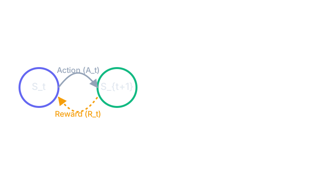
An MDP formalizes sequential decision-making: an agent in a state takes an action, receives a reward, and transitions to a new state, with the goal of maximizing cumulative discounted reward over time.

Why Does This Exist?

To train an agent to make decisions over time, you need a mathematical model: what states exist, what actions are available, what happens when you take an action, and what reward you receive. The Markov Decision Process provides exactly this framework — the foundation on which every reinforcement learning algorithm builds.

MDPs formalize a deceptively simple scenario: an agent repeatedly chooses actions, receives rewards, and observes state transitions. The catch is that consequences can be delayed — a chess move that looks brilliant now might cost you the game ten moves later. The MDP gives you the mathematics to reason about these delayed consequences.

Think of It Like This

Navigating a city with traffic lights

Your state is your current position. Actions are turning choices (left, right, straight). Each action takes you to a new position — possibly with a traffic delay (stochastic transition). The reward is your travel time (negative: shorter is better). Your goal is to find the route — the policy — that minimizes total travel time, accounting for all future intersections you'll encounter.

How It Actually Works

The five-tuple definition

An MDP is defined by $(S, A, T, R, \gamma)$ :

Symbol	Name	Meaning
$S$	State space	All possible situations the agent can be in
$A$	Action space	All possible actions the agent can take
$T(s' \mid s, a)$	Transition function	Probability of reaching $s'$ from $s$ after $a$
$R(s, a, s')$	Reward function	Immediate reward for transition $(s, a, s')$
$\gamma \in [0,1]$	Discount factor	How much future rewards are discounted

The Markov property

The future depends only on the current state, not on the history of how you arrived there:

$P(s_{t+1} \mid s_0, a_0, \ldots, s_t, a_t) = P(s_{t+1} \mid s_t, a_t) = T(s_{t+1} \mid s_t, a_t)$

This assumption makes the math tractable — the agent doesn't need to remember the full history of actions taken.

Policy and value functions

A policy $\pi(a \mid s)$ maps states to a distribution over actions (or deterministically to one action). The value function $V^\pi(s)$ is the expected discounted return when starting from state $s$ and following $\pi$ :

$V^\pi(s) = \mathbb{E}_\pi\left[\sum_{t=0}^{\infty} \gamma^t R_t \;\Big|\; s_0 = s\right]$

The action-value function $Q^\pi(s, a)$ extends this to evaluate specific actions:

$Q^\pi(s, a) = \mathbb{E}_\pi\left[\sum_{t=0}^{\infty} \gamma^t R_t \;\Big|\; s_0 = s, a_0 = a\right]$

Bellman equations

The Bellman equations express value functions recursively:

$V^\pi(s) = \sum_a \pi(a \mid s) \sum_{s'} T(s' \mid s, a)\left[R(s, a, s') + \gamma V^\pi(s')\right]$

The Bellman optimality equations characterize the optimal value function $V^*$ :

$V^*(s) = \max_a \sum_{s'} T(s' \mid s, a)\left[R(s, a, s') + \gamma V^*(s')\right]$

Solving small MDPs: value iteration

For small discrete MDPs, value iteration repeatedly applies the Bellman optimality operator until convergence:

1V(s) ← max_a Σ_s' T(s'|s,a)[R(s,a,s') + γV(s')]   for all s

This converges to $V^*$ in a finite number of iterations for finite MDPs with $\gamma < 1$ .

Code

1import numpy as np2
3# ── Gridworld MDP: 4×4 grid, goal at state 15, holes at 5 and 13 ─────────────4# States: 0-15 (row-major). Actions: 0=up, 1=right, 2=down, 3=left5# Transitions: deterministic (simplification; real FrozenLake is stochastic)6
7NUM_STATES = 168NUM_ACTIONS = 49GAMMA = 0.9510
11def get_transitions(s, a):12    """Returns list of (next_state, reward, done) for deterministic gridworld."""13    row, col = divmod(s, 4)14    if s in [5, 13, 15]:  # holes and goal are terminal15        return [(s, 0.0, True)]16    17    dr, dc = [(-1,0),(0,1),(1,0),(0,-1)][a]18    nr, nc = row + dr, col + dc19    # Bounce off walls20    if 0 <= nr < 4 and 0 <= nc < 4:21        ns = nr * 4 + nc22    else:23        ns = s  # stay in place24    25    if ns == 15:26        reward = 10.027    elif ns in [5, 13]:28        reward = -10.029    else:30        reward = -1.0  # step cost31    32    done = ns in [5, 13, 15]33    return [(ns, reward, done)]34
35# Value iteration36V = np.zeros(NUM_STATES)37for iteration in range(500):38    V_new = V.copy()39    for s in range(NUM_STATES):40        if s in [5, 13, 15]:  # terminal states41            V_new[s] = 0.042            continue43        q_values = []44        for a in range(NUM_ACTIONS):45            q = sum(prob * (r + GAMMA * V[ns] * (1 - int(done)))46                    for ns, r, done in get_transitions(s, a)47                    for prob in [1.0])48            q_values.append(q)49        V_new[s] = max(q_values)50    51    if np.max(np.abs(V_new - V)) < 1e-6:52        print(f"Converged after {iteration+1} iterations")53        break54    V = V_new55
56print("Optimal value function:")57print(V.reshape(4, 4).round(1))58
59# Derive greedy policy60policy = []61for s in range(NUM_STATES):62    if s in [5, 13, 15]:63        policy.append(-1)64        continue65    q_values = [sum(r + GAMMA * V[ns] * (1 - int(done))66                    for ns, r, done in get_transitions(s, a))67                for a in range(NUM_ACTIONS)]68    policy.append(int(np.argmax(q_values)))69
70action_names = ['↑', '→', '↓', '←']71print("\nOptimal policy:")72for row in range(4):73    print(" ".join(action_names[policy[row*4+col]] if policy[row*4+col] >= 0 else 'X'74                   for col in range(4)))

Watch Out For

The curse of dimensionality

Value iteration and policy iteration enumerate all states. With 20 binary features, the state space has $2^{20} \approx 10^6$ states — manageable. With 100 continuous sensors, it's infinite and completely intractable. Real-world RL uses function approximation (neural networks) to generalize across states rather than tabulating them all. The MDP framework still applies; only the solution method changes.

Reward hacking from misspecified rewards

An RL agent optimizes the reward you give it, not the reward you meant to give it. A cleaning robot rewarded for maximizing covered area may learn to move in circles. A game-playing agent rewarded for score may exploit bugs. Reward design is the central alignment challenge: specify what you actually want, not a convenient proxy.

The Quick Version

An MDP = $(S, A, T, R, \gamma)$ : states, actions, transition function, reward function, discount.
The Markov property: future depends only on the current state, not history. Makes the math tractable.
Policy $\pi$ maps states to actions; the value function $V^\pi(s)$ measures expected discounted return.
Bellman equations express value recursively; value iteration solves them for small discrete MDPs.
Large/continuous state spaces require neural function approximation — this is where DQN and actor-critic methods come in.