Optimistic Initial Values

By initializing action values far above realistic rewards, an agent is naturally disappointed every time it tries an action, systematically driving it to sample all untried alternatives.

Why Does This Exist?

In reinforcement learning, a standard greedy action-selection policy ( $\varepsilon = 0$ ) chooses whichever action currently has the highest estimated value. If all action-value estimates are initialized to zero ( $Q_1(a) = 0$ ), the agent falls victim to an immediate lock-in trap: the first arm it samples that produces any positive reward (e.g., $+0.2$ ) instantly becomes the highest-rated option. Untried arms remain at $0.0$ , so the greedy agent exploits that mediocre arm indefinitely, never discovering that a neighboring arm yields $+0.8$ .

Without an active exploration mechanism, greedy agents suffer severe lock-in and catastrophic regret. While $\varepsilon$ -greedy prevents this by injecting random action selection, it carries a persistent tax: the agent continues pulling suboptimal arms at a fixed random rate $\varepsilon$ forever, unless a complex decay schedule is hand-tuned.

Optimistic initial values provide a simple, deterministic exploration technique for stationary tabular problems. By deliberately setting the starting estimates well above any achievable reward ( $Q_1(a) \gg R_{\max}$ ), every action taken produces an outcome lower than expected. This systematic disappointment depresses the chosen arm's estimate below the pristine estimates of untried arms, naturally compelling the greedy policy to sample every available action before repeating any of them.

Think of It Like This

The Hyper-Optimistic Restaurant Critic

Imagine a food critic who moves to a new city and starts with an unshakable assumption: every restaurant in this city is a 5-star culinary masterpiece until proven otherwise.

On Monday evening, seeking dinner, the critic visits Restaurant A (expected rating: 5.0 stars). The meal is respectable—a 3-star dinner. Because 3 stars is lower than their 5.0-star expectation, the critic feels disappointed and lowers Restaurant A's mental rating to 4.2 stars.

On Tuesday evening, the critic asks: "Where is the best place to eat?" Restaurant A is now rated 4.2 stars, but Restaurants B, C, and D are still assumed to be 5.0 stars. Being purely greedy (always picking the highest-rated venue), the critic walks past Restaurant A and dines at Restaurant B. Restaurant B turns out to be a greasy spoon that serves a 1-star meal, plunging its rating to 3.8 stars.

On Wednesday and Thursday, the critic visits Restaurants C and D because untried eateries still hold the pristine 5.0-star rating.

The critic never needs to flip a coin or pick restaurants at random. Their initial optimism guarantees that every early meal brings disappointment, automatically driving them to tour every eatery in town before settling down on the true best spot.

Where the analogy stops: In real life, restaurants change owners, hire new chefs, or overhaul menus over time (non-stationarity). If Restaurant B hires a Michelin-starred chef a year later, the critic—whose rating for Restaurant B is permanently parked at 1.8 stars—will never step inside again. Optimism only burns once; it does not rekindle when the environment changes.

How It Actually Works

The Mechanism of Systematic Disappointment

Let $\mathcal{A} = \{1, 2, \dots, k\}$ denote the discrete action set, and let rewards be bounded such that $R_t \in [R_{\min}, R_{\max}]$ .

The agent maintains an action-value estimate $Q_t(a)$ for each action $a \in \mathcal{A}$ . At step $t$ , a purely greedy policy selects the action with the maximum estimated value:

$A_t = \arg\max_{a \in \mathcal{A}} Q_t(a)$

When ties occur, they are broken deterministically (e.g., choosing the lowest index). After executing action $A_t$ and observing reward $R_t$ , the estimate is updated via a constant step-size parameter $\alpha \in (0, 1]$ :

$Q_{t+1}(A_t) = Q_t(A_t) + \alpha \big[ R_t - Q_t(A_t) \big]$

where:

$Q_t(A_t)$ is the prior value estimate for the selected action.
$R_t$ is the observed scalar reward.
$[R_t - Q_t(A_t)]$ is the prediction error (surprise).
$\alpha$ is the constant step-size parameter (learning rate).

Under optimistic initialization, the initial values are configured such that:

$Q_1(a) = Q_0 > R_{\max}, \quad \forall a \in \mathcal{A}$

Because every realized reward satisfies $R_t \le R_{\max} < Q_0$ , the prediction error on the initial selection of any arm is guaranteed to be negative:

$R_t - Q_t(A_t) < 0 \implies Q_{t+1}(A_t) < Q_t(A_t)$

The chosen arm's estimate immediately drops below $Q_0$ . Meanwhile, all untested arms retain their optimistic ceiling of $Q_0$ . At step $t + 1$ , the greedy rule strictly prefers the untried actions over the sampled action.

Expanding the constant step-size update rule recursively shows how initial optimism decays over $n$ selections of an action:

$Q_{n+1}(a) = (1 - \alpha)^n Q_1(a) + \sum_{i=1}^n \alpha (1 - \alpha)^{n-i} R_i$

The initial value $Q_1(a)$ acts as a prior whose influence decays at an exponential rate of $(1 - \alpha)^n$ . As $n \to \infty$ , $(1 - \alpha)^n \to 0$ , eliminating the initial bias and allowing $Q(a)$ to converge to the true expected reward $\mu_a$ .

Worked numerical example

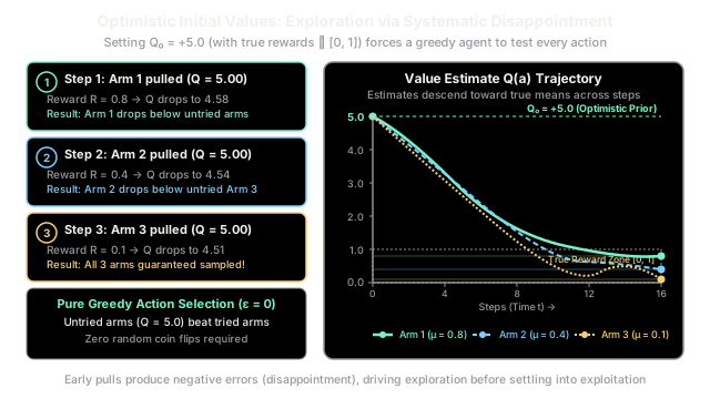
Consider a 3-armed bandit ( $k = 3$ ) with true reward means $\mu_1 = 0.80$ , $\mu_2 = 0.40$ , and $\mu_3 = 0.10$ . Let the learning rate be $\alpha = 0.10$ , and initialize all arms optimistically to $Q_1(a) = 5.00$ . When multiple arms share the maximal value, the tie is broken by choosing the smallest arm index.

Step 1 ( $t = 1$ ):
- Current estimates: $Q_1 = [5.00, 5.00, 5.00]$ .
- Selection: All three arms are tied at $5.00$ . Smallest index selects Arm 1 ( $A_1 = 1$ ).
- Observed reward: $R_1 = 0.80$ .
- Prediction error: $R_1 - Q_1(1) = 0.80 - 5.00 = -4.20$ .
- Update: $Q_2(1) = 5.00 + 0.10 \times (-4.20) = 5.00 - 0.42 = 4.58$
- New estimates: $Q_2 = [4.58, 5.00, 5.00]$ .
- Outcome: Disappointment lowers Arm 1 below the untried arms.
Step 2 ( $t = 2$ ):
- Current estimates: $Q_2 = [4.58, 5.00, 5.00]$ .
- Selection: Arms 2 and 3 are tied at $5.00 > 4.58$ . Smallest index selects Arm 2 ( $A_2 = 2$ ).
- Observed reward: $R_2 = 0.40$ .
- Prediction error: $R_2 - Q_2(2) = 0.40 - 5.00 = -4.60$ .
- Update: $Q_3(2) = 5.00 + 0.10 \times (-4.60) = 5.00 - 0.46 = 4.54$
- New estimates: $Q_3 = [4.58, 4.54, 5.00]$ .
- Outcome: Arm 2 drops to $4.54$ . Untried Arm 3 is now uniquely highest.
Step 3 ( $t = 3$ ):
- Current estimates: $Q_3 = [4.58, 4.54, 5.00]$ .
- Selection: Arm 3 uniquely maximizes $Q$ ( $5.00 > 4.58 > 4.54$ ), so $A_3 = 3$ .
- Observed reward: $R_3 = 0.10$ .
- Prediction error: $R_3 - Q_3(3) = 0.10 - 5.00 = -4.90$ .
- Update: $Q_4(3) = 5.00 + 0.10 \times (-4.90) = 5.00 - 0.49 = 4.51$
- New estimates: $Q_4 = [4.58, 4.54, 4.51]$ .
- Outcome: Every arm has now been sampled once without any random exploration.
Step 4 ( $t = 4$ ):
- Current estimates: $Q_4 = [4.58, 4.54, 4.51]$ .
- Selection: Arm 1 has the highest estimate ( $4.58$ ) because it suffered the smallest disappointment ( $R = 0.80$ ). The agent selects $A_4 = 1$ .
- Observed reward: $R_4 = 0.80$ .
- Prediction error: $R_4 - Q_4(1) = 0.80 - 4.58 = -3.78$ .
- Update: $Q_5(1) = 4.58 + 0.10 \times (-3.78) = 4.58 - 0.378 = 4.202$
- New estimates: $Q_5 = [4.202, 4.54, 4.51]$ .
- Outcome: Arm 1 drops to $4.202$ , falling below Arm 2 ( $4.54$ ) and Arm 3 ( $4.51$ ). On Step 5, the greedy policy naturally switches back to Arm 2, cycling through multiple passes across all arms until value estimates converge to the true reward range.

Code

1def simulate_greedy_bandit(2    true_means: list[float],3    initial_q: float,4    steps: int = 12,5    alpha: float = 0.2,6) -> tuple[list[int], list[float]]:7    """Simulates a greedy bandit agent with given initial Q-values."""8    num_arms = len(true_means)9    q_values = [initial_q] * num_arms10    action_history: list[int] = []11
12    for _ in range(steps):13        # Pure greedy action selection (break ties by lowest index)14        best_arm = 015        best_val = q_values[0]16        for arm in range(1, num_arms):17            if q_values[arm] > best_val:18                best_val = q_values[arm]19                best_arm = arm20
21        # Observe reward and update value estimate22        reward = true_means[best_arm]23        q_values[best_arm] += alpha * (reward - q_values[best_arm])24        action_history.append(best_arm)25
26    return action_history, [round(v, 3) for v in q_values]27
28
29# Arm 0 is mediocre (0.2), Arm 1 is optimal (0.8), Arm 2 is poor (0.1)30true_means = [0.2, 0.8, 0.1]31
32# 1. Standard zero initialization (Q0 = 0.0) -> Trapped on mediocre Arm 033zero_actions, zero_q = simulate_greedy_bandit(true_means, initial_q=0.0)34
35# 2. Optimistic initialization (Q0 = 5.0) -> Explores all arms systematically36opt_actions, opt_q = simulate_greedy_bandit(true_means, initial_q=5.0)37
38print(f"Zero-init actions:       {zero_actions}")39# -> Zero-init actions:       [0, 0, 0, 0, 0, 0, 0, 0, 0, 0, 0, 0]40
41print(f"Zero-init final Q:       {zero_q}")42# -> Zero-init final Q:       [0.186, 0.0, 0.0]43
44print(f"Optimistic actions:      {opt_actions}")45# -> Optimistic actions:      [0, 1, 2, 1, 0, 2, 1, 0, 2, 1, 0, 2]46
47print(f"Optimistic final Q:      {opt_q}")48# -> Optimistic final Q:      [2.166, 2.52, 2.107]

Watch Out For

Failure in Non-Stationary Environments

Optimistic initial values only produce transient exploration. Once the initial optimistic bias decays ( $(1 - \alpha)^n \approx 0$ ) and all arms have been sampled multiple times, the mechanism completely ceases to drive exploration.

If the environment is non-stationary—meaning reward distributions drift over time or a previously weak arm becomes the new optimal option later in the run—a purely greedy agent will never detect the shift. Because its estimate for that arm is already depressed and initial optimism has vanished, the agent stays permanently locked onto its historical favorite.

The Fix: Never use optimistic initial values as the sole exploration mechanism in non-stationary problems. Combine optimism with continuous exploration strategies such as $\varepsilon$ -greedy with a persistent floor, Upper Confidence Bound (UCB) with sliding observation windows, or discounted tracking updates.

Excessive Exploration from Oversized Initial Values

If initial values $Q_0$ are set unrealistically high relative to the step size $\alpha$ , the optimistic bias $(1 - \alpha)^n Q_0$ takes an exorbitant number of steps to decay. The agent will repeatedly sample obviously terrible arms across hundreds of rounds simply because their estimates remain artificially inflated well above reality.

The Fix: Set $Q_0$ only modestly above the known upper bound of rewards (e.g., $Q_0 \approx 1.5 \times R_{\max}$ to $2 \times R_{\max}$ ). Avoid arbitrarily huge initializations like $Q_0 = +1000$ unless accompanied by a proportionally large early learning rate.

The Quick Version

Core Mechanism: Action-value estimates are initialized to an optimistic ceiling ( $Q_1(a) \gg R_{\max}$ ) well above any achievable reward.
Exploration via Disappointment: Every trial produces negative surprise ( $R_t - Q_t(A_t) < 0$ ), depressing that action's estimate and forcing a greedy policy ( $\varepsilon = 0$ ) to try untried alternatives.
Deterministic Efficiency: Unlike $\varepsilon$ -greedy, exploration is structured and non-random, eliminating wasted pulls on random actions once estimates converge.
Transient Exploration Only: Initial optimism burns away once tested; it cannot adapt to non-stationary environments where optimal arms drift over time.