Policy Gradient Methods
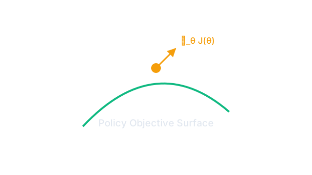
Policy gradient methods directly optimize the policy by estimating the gradient of expected reward with respect to policy parameters, making them applicable to continuous action spaces where value-based methods struggle.
Why Does This Exist?
Q-learning selects actions via . When the action space is continuous — robot joint angles, throttle levels, portfolio weights, drug dosages — this argmax is intractable. Policy gradient methods sidestep this entirely by directly parameterizing the policy and optimizing it via gradient ascent.
A second motivation: stochastic policies. Value-based methods produce deterministic greedy policies. But some tasks require mixed strategies — a deterministic policy in rock-paper-scissors is exploitable. Policy gradient naturally represents and learns stochastic policies.
Think of It Like This
A chef adjusting a recipe based on diner feedback
A chef adjusting a recipe doesn't consult a fixed lookup table of optimal spice ratios. They cook a dish, collect feedback ("too salty", "a bit bland"), and nudge the recipe slightly in the direction that diners preferred. Over many meals and feedback cycles, the recipe converges toward something diners love. REINFORCE does exactly this: collect trajectories, observe which actions led to high returns, and nudge policy parameters to make those actions more probable.
How It Actually Works
The policy gradient theorem
We want to maximize expected return . The policy gradient theorem gives:
Where is the return from timestep .
The key term is the score function: it points in the direction that increases the probability of action in state . Multiplying by means: if (good outcome), push toward ; if (bad outcome), push away from it.
REINFORCE (Monte Carlo policy gradient)
The simplest policy gradient algorithm:
- Sample trajectory under current
- Compute returns for each timestep
- Update:
Variance reduction with a baseline
The REINFORCE gradient estimator has high variance — returns vary dramatically across episodes. Subtracting a baseline that doesn't depend on leaves the gradient unbiased while reducing variance:
The baseline is typically , estimated by a separate value network. The advantage measures how much better action was compared to what was expected on average in state .
Policy parameterization
- Discrete actions: Softmax over learned logits —
- Continuous actions: Gaussian policy — , where the network outputs mean and log-std
Code
import gymnasium as gymimport torchimport torch.nn as nnimport torch.optim as optim
# ── Policy network (discrete actions) ────────────────────────────────────────class PolicyNet(nn.Module): def __init__(self, obs_dim, n_actions, hidden=128): super().__init__() self.net = nn.Sequential( nn.Linear(obs_dim, hidden), nn.ReLU(), nn.Linear(hidden, hidden), nn.ReLU(), nn.Linear(hidden, n_actions), ) def forward(self, x): return torch.softmax(self.net(x), dim=-1)
# ── REINFORCE with baseline ───────────────────────────────────────────────────env = gym.make("CartPole-v1")obs_dim = env.observation_space.shape[0]n_actions = env.action_space.n
policy = PolicyNet(obs_dim, n_actions)baseline = nn.Sequential(nn.Linear(obs_dim, 128), nn.ReLU(), nn.Linear(128, 1))opt_p = optim.Adam(policy.parameters(), lr=3e-4)opt_b = optim.Adam(baseline.parameters(), lr=1e-3)
gamma = 0.99
for episode in range(800): states, actions, rewards = [], [], [] state, _ = env.reset() done = False
while not done: s_tensor = torch.tensor(state, dtype=torch.float32) probs = policy(s_tensor) action = torch.multinomial(probs, 1).item() next_state, reward, terminated, truncated, _ = env.step(action) states.append(state); actions.append(action); rewards.append(reward) state = next_state done = terminated or truncated
# Compute discounted returns G, returns = 0.0, [] for r in reversed(rewards): G = r + gamma * G returns.insert(0, G) returns = torch.tensor(returns, dtype=torch.float32)
states_t = torch.tensor(states, dtype=torch.float32) actions_t = torch.tensor(actions, dtype=torch.long)
# Baseline update (value regression) values = baseline(states_t).squeeze() baseline_loss = nn.MSELoss()(values, returns) opt_b.zero_grad(); baseline_loss.backward(); opt_b.step()
# Policy update (REINFORCE with advantage) with torch.no_grad(): advantages = returns - baseline(states_t).squeeze()
# Normalize advantages for stability advantages = (advantages - advantages.mean()) / (advantages.std() + 1e-8)
log_probs = torch.log(policy(states_t).gather(1, actions_t.unsqueeze(1)).squeeze() + 1e-8) policy_loss = -(log_probs * advantages).mean() opt_p.zero_grad(); policy_loss.backward(); opt_p.step()
if episode % 100 == 0: ep_return = sum(rewards) print(f"Episode {episode:>4}: return={ep_return:.0f}, steps={len(rewards)}")
env.close()Watch Out For
High variance of Monte Carlo gradient estimates
Monte Carlo returns are noisy — the same policy produces very different return values due to environment stochasticity and long episode horizons. This makes REINFORCE slow and unstable. Use a baseline (as above), or move to actor-critic methods that use bootstrapped value estimates () instead of Monte Carlo returns for lower variance.
Large policy updates destroying good behavior
A large gradient update can move the policy far from its current position, collapsing it (assigning probability 1 to one action) or making it worse. This is the motivation for PPO (Proximal Policy Optimization), which clips the probability ratio to prevent large updates: .
The Quick Version
- Policy gradients directly optimize via .
- REINFORCE: collect Monte Carlo trajectories, compute returns, update policy — simple but high variance.
- Baselines reduce variance: advantage keeps the gradient unbiased while reducing noise.
- Works with continuous actions and naturally represents stochastic policies (unlike Q-learning).
- PPO and TRPO extend policy gradient with update-size constraints for stability.