Q-Learning

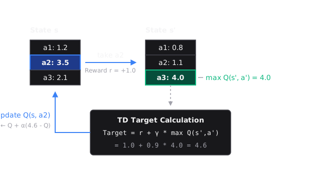
Q-learning estimates the value of taking each action in each state without needing a model of the environment, converging to the optimal action-value function by bootstrapping off its own past estimates.

Why Does This Exist?

Most real-world problems don't give you the transition model $T(s' \mid s, a)$ or reward function $R(s, a, s')$ in closed form — you can only observe the outcomes of actions you actually take. Q-learning is model-free: it learns optimal action values purely from experience, without ever knowing the environment dynamics.

This is the key breakthrough: you don't need to know how the world works. You just need to interact with it.

Think of It Like This

Learning which moves win at chess by playing

You learn to play chess not by memorizing a complete game tree, but by playing thousands of games and remembering which positions tended to lead to wins. After enough games, your estimate of how good each position is becomes accurate. Q-learning does exactly this: maintain a running estimate of how valuable each action is in each state, and update that estimate after every move based on what actually happened.

How It Actually Works

The Q-function

The Q-function $Q(s, a)$ estimates the expected discounted return of taking action $a$ in state $s$ , then following the optimal policy thereafter. The optimal Q-function $Q^*$ satisfies the Bellman optimality equation:

$Q^*(s, a) = \mathbb{E}\left[R + \gamma \max_{a'} Q^*(s', a') \;\Big|\; s, a\right]$

If we know $Q^*$ , the optimal policy is simply: in state $s$ , take $\arg\max_a Q^*(s, a)$ .

The Q-update rule

After observing transition $(s, a, r, s')$ :

$Q(s, a) \leftarrow Q(s, a) + \alpha\underbrace{\left[r + \gamma \max_{a'} Q(s', a') - Q(s, a)\right]}_{\text{TD error}}$

The TD error is the difference between the bootstrapped target ( $r + \gamma \max_{a'} Q(s', a')$ ) and the current estimate. A positive TD error means the current estimate is too low — increase it. A negative error means it's too high — decrease it. $\alpha$ is the learning rate.

Off-policy learning

Q-learning is off-policy: the target uses $\max_{a'} Q(s', a')$ (the greedy action) regardless of which action the agent actually took during exploration. This means the agent can explore with $\varepsilon$ -greedy (taking random actions $\varepsilon$ of the time) while still learning the optimal policy — the exploration policy and the target policy are decoupled.

Convergence guarantee

For tabular Q-learning with finite state-action spaces, $Q$ converges to $Q^*$ if:

Every state-action pair is visited infinitely often.
Learning rates satisfy $\sum_t \alpha_t = \infty$ (enough total learning) and $\sum_t \alpha_t^2 < \infty$ (learning slows over time).

In practice: use a small constant $\alpha$ (e.g., 0.1) and anneal $\varepsilon$ from 1.0 to 0.01.

Code

1import gymnasium as gym2import numpy as np3
4# ── Tabular Q-learning on FrozenLake ─────────────────────────────────────────5env = gym.make("FrozenLake-v1", is_slippery=True, render_mode=None)6num_states  = env.observation_space.n   # 167num_actions = env.action_space.n         # 48
9# Initialize Q-table10Q = np.zeros((num_states, num_actions))11
12# Hyperparameters13alpha   = 0.1    # learning rate14gamma   = 0.99   # discount factor15epsilon = 1.0    # initial exploration rate16eps_min = 0.01   # minimum exploration rate17eps_decay = 0.99918
19rewards_per_episode = []20
21for episode in range(10_000):22    state, _ = env.reset()23    total_reward = 0.024    done = False25
26    while not done:27        # ε-greedy action selection28        if np.random.random() < epsilon:29            action = env.action_space.sample()   # explore30        else:31            action = np.argmax(Q[state])          # exploit32
33        next_state, reward, terminated, truncated, _ = env.step(action)34        done = terminated or truncated35
36        # Q-update (Bellman target)37        td_target = reward + gamma * np.max(Q[next_state]) * (1 - int(terminated))38        td_error  = td_target - Q[state, action]39        Q[state, action] += alpha * td_error40
41        state = next_state42        total_reward += reward43
44    # Anneal exploration45    epsilon = max(eps_min, epsilon * eps_decay)46    rewards_per_episode.append(total_reward)47
48# Evaluation (greedy policy, no exploration)49eval_rewards = []50for _ in range(100):51    state, _ = env.reset()52    total = 0.053    done = False54    while not done:55        action = np.argmax(Q[state])56        state, reward, terminated, truncated, _ = env.step(action)57        done = terminated or truncated58        total += reward59    eval_rewards.append(total)60
61print(f"Greedy policy win rate: {np.mean(eval_rewards):.1%}")62print("\nLearned Q-values (action with highest Q per state):")63print(np.argmax(Q, axis=1).reshape(4, 4))  # 0=L, 1=D, 2=R, 3=U

Watch Out For

Overestimation bias in the Q-target

The target $\max_{a'} Q(s', a')$ uses the maximum of noisy Q-estimates, which is systematically biased upward — the maximum of noisy values overestimates the true maximum. This overestimation accumulates and can cause instability or suboptimal convergence. Double Q-learning addresses this: use one network to select $a^* = \arg\max_{a'} Q_1(s', a')$ and a second network to evaluate $Q_2(s', a^*)$ , eliminating the bias.

Not visiting enough state-action pairs

Q-learning converges only when every state-action pair is visited sufficiently. With aggressive $\varepsilon$ annealing, the agent commits to a nearly greedy policy before it has explored enough states. Monitor a visitation heatmap — if many states have near-zero visit counts when $\varepsilon$ is already small, slow the annealing schedule.

The Quick Version

Q-learning is model-free and off-policy: learns the optimal action-value function directly from experience.
The Q-update: $Q(s,a) \leftarrow Q(s,a) + \alpha[r + \gamma\max_{a'} Q(s',a') - Q(s,a)]$ .
Off-policy: the target uses the greedy action regardless of the exploration policy used during data collection.
Tabular convergence guaranteed when all state-action pairs visited sufficiently with decaying learning rates.
Doesn't scale to large/continuous state spaces → needs neural network approximation (DQN).