Upper Confidence Bound (UCB)

Optimism in the face of uncertainty: estimate each action's potential payout plus an uncertainty bonus, picking whichever candidate could plausibly be the best.

The Upper Confidence Bound algorithm balances exploitation and exploration by augmenting sample averages with an uncertainty bonus.

Why Does This Exist?

In the multi-armed bandit problem, an agent must choose among actions with unknown reward distributions to maximize cumulative payoff. If the agent acts greedily—always picking the arm with the highest observed average—it can easily become trapped in a suboptimal choice because an arm that initially produced an unlucky low reward might never be sampled again.

Heuristic alternatives like epsilon-greedy address this by picking a random action with probability $\varepsilon$ . However, $\varepsilon$ -greedy explores blindly: it treats an action that is proven to be disastrous with the exact same probability as an action that has never been tried and might be outstanding.

The Upper Confidence Bound (UCB) algorithm solves this by formalizing optimism in the face of uncertainty. Instead of exploring at random, UCB assigns each action an exploration bonus proportional to how uncertain its true payoff remains. An action is selected if either its empirical mean is high (exploitation) or its uncertainty interval is wide (directed exploration). As an action is chosen more frequently, its uncertainty interval contracts, naturally phasing out exploration without manual tuning of decay schedules and guaranteeing asymptotically optimal logarithmic regret $O(\ln T)$ .

Think of It Like This

Evaluating experimental medical treatments in a clinical trial

Imagine a doctor evaluating three experimental therapies for a rare disease:

Treatment A has been administered to 50 patients with a 70% remission rate.
Treatment B has been administered to 20 patients with a 65% remission rate.
Treatment C is brand new and has only been administered to 2 patients, with 1 remission (50% empirical remission rate).

If the doctor behaves purely greedily, they will only administer Treatment A, permanently ignoring Treatment C. If they follow an $\varepsilon$ -greedy policy, they will arbitrarily assign random treatments to 10% of future patients—even if a therapy is known to perform poorly.

Under the Upper Confidence Bound principle, the doctor calculates the maximum plausible success rate (an upper confidence interval) for each option. For Treatment A, 50 trials provide high statistical certainty: its true success rate plausibly lies between 60% and 80%. For Treatment C, only 2 trials exist, meaning extreme uncertainty: its true success rate could plausibly be anywhere from 10% to 95%.

Because Treatment C has an upper plausible bound of 95% (higher than Treatment A's 80%), the doctor selects Treatment C next. If Treatment C fails a few more times, its uncertainty interval rapidly shrinks, pulling its upper bound below Treatment A. If it succeeds, the doctor discovers a superior treatment.

Where the analogy stops: In medical trials, strict institutional review boards, ethical constraints, and phased testing restrict dynamic real-time reallocation. Bandit algorithms assume the agent is free to pull any available arm at each discrete decision step.

How It Actually Works

Mathematical Formulation and the UCB1 Rule

Let $K$ denote the number of actions (arms). At each discrete time step $t \in \{1, 2, \dots, T\}$ , the agent selects an action $A_t = a$ and receives a scalar reward $R_t \in [0, 1]$ .

We track two quantities for every arm $a$ :

$N_t(a)$ : the number of times arm $a$ was selected prior to step $t$ .
$Q_t(a)$ : the sample average reward obtained from arm $a$ prior to step $t$ :

$Q_t(a) = \frac{1}{N_t(a)} \sum_{i=1}^{t-1} R_i \cdot \mathbb{I}(A_i = a)$

The standard UCB1 decision rule selects the action that maximizes the sum of the empirical mean and an uncertainty bonus:

$A_t = \arg\max_{a} \left[ Q_t(a) + c \sqrt{\frac{\ln t}{N_t(a)}} \right]$

where:

$Q_t(a)$ is the exploitation component representing the current estimated value of arm $a$ .
$c \sqrt{\frac{\ln t}{N_t(a)}}$ is the exploration bonus (uncertainty bound) $U_t(a)$ .
$t$ is the total number of time steps elapsed across all arms. The numerator $\ln t$ grows over time, which slowly increases the exploration bonus for arms that are not being selected, preventing any arm from being permanently abandoned.
$N_t(a)$ is in the denominator under the square root. Every time arm $a$ is pulled, $N_t(a)$ increments, which shrinks its uncertainty bonus and demands higher empirical performance for future selection.
$c > 0$ is an exploration coefficient that governs the agent's confidence level. In the canonical UCB1 derivation, $c = \sqrt{2} \approx 1.414$ .

Statistical Basis: Hoeffding's Inequality

The square-root bonus is derived directly from Hoeffding's Inequality, which bounds the probability that the empirical sample mean $Q_t(a)$ underestimates the true expected value $\mu_a$ for bounded random variables $R \in [0, 1]$ :

$P\left( \mu_a > Q_t(a) + U \right) \le \exp\left( -2 N_t(a) U^2 \right)$

Setting the upper tail probability to $p = t^{-4}$ and solving for the uncertainty margin $U$ :

$t^{-4} = \exp\left( -2 N_t(a) U^2 \right) \implies U = \sqrt{\frac{2 \ln t}{N_t(a)}}$

This guarantees that the true mean $\mu_a$ lies below $Q_t(a) + \sqrt{\frac{2 \ln t}{N_t(a)}}$ with probability at least $1 - t^{-4}$ . As $t$ increases, the failure probability decays rapidly. Auer, Cesa-Bianchi, and Fischer (2002) proved that UCB1 achieves logarithmic cumulative regret:

$\mathbb{E}[\text{Regret}(T)] \le O(\ln T)$

This matches the theoretical lower bound proved by Lai and Robbins (1985).

Worked numerical example

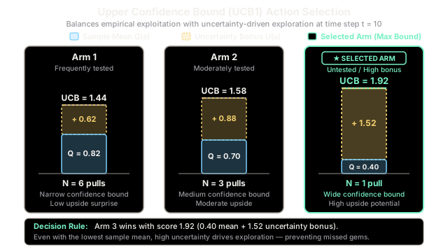
Consider a 3-armed bandit problem at time step $t = 10$ with exploration coefficient $c = 1.0$ .

Across the previous 9 time steps, the agent has collected the following statistics:

Arm 1: $N_{10}(1) = 6$ pulls, sample average $Q_{10}(1) = 0.82$
Arm 2: $N_{10}(2) = 3$ pulls, sample average $Q_{10}(2) = 0.70$
Arm 3: $N_{10}(3) = 1$ pull, sample average $Q_{10}(3) = 0.40$
Total pulls: $N_1 + N_2 + N_3 = 6 + 3 + 1 = 10 = t$ .

We compute $\ln(t) = \ln(10) \approx 2.3026$ .

Step 1: Compute the exploration bonus $U_{10}(a) = c \sqrt{\frac{\ln t}{N_t(a)}}$ for each arm:

Arm 1: $U_{10}(1) = 1.0 \times \sqrt{\frac{2.3026}{6}} = \sqrt{0.3838} \approx 0.620$
Arm 2: $U_{10}(2) = 1.0 \times \sqrt{\frac{2.3026}{3}} = \sqrt{0.7675} \approx 0.876$
Arm 3: $U_{10}(3) = 1.0 \times \sqrt{\frac{2.3026}{1}} = \sqrt{2.3026} \approx 1.517$

Step 2: Compute the total Upper Confidence Bound score $Q_{10}(a) + U_{10}(a)$ :

Arm 1: $\text{UCB}(1) = 0.82 + 0.620 = 1.440$
Arm 2: $\text{UCB}(2) = 0.70 + 0.876 = 1.576$
Arm 3: $\text{UCB}(3) = 0.40 + 1.517 = 1.917$

Step 3: Select the action with the maximum UCB score:

$A_{10} = \arg\max_{a} \{1.440, 1.576, 1.917\} = \text{Arm } 3$

Despite having the lowest empirical average ( $0.40$ versus Arm 1's $0.82$ ), Arm 3 is selected. Its single trial carries substantial uncertainty, producing a bonus of $+1.517$ that pushes its plausible upper bound above all competitors.

If the agent pulls Arm 3 at $t = 10$ and receives a reward of $0.0$ :

Its new sample average drops to $Q_{11}(3) = \frac{0.40 + 0.0}{2} = 0.20$ .
Its pull count increments to $N_{11}(3) = 2$ .
At $t = 11$ , its bonus contracts to $\sqrt{\frac{\ln 11}{2}} = \sqrt{\frac{2.3979}{2}} \approx 1.095$ .
Its new score becomes $0.20 + 1.095 = 1.295$ .

Arm 2 and Arm 1 now surpass Arm 3, demonstrating how testing an uncertain option automatically extinguishes unpromising exploration.

Code

The following implementation executes the UCB1 algorithm over a multi-armed bandit simulation with type annotations and standard library dependencies:

1import math2import random3from typing import List4
5class UCB1Bandit:6    """Multi-armed bandit solver using the Upper Confidence Bound (UCB1) algorithm."""7
8    def __init__(self, n_arms: int, c: float = 1.414) -> None:9        self.n_arms: int = n_arms10        self.c: float = c11        self.counts: List[int] = [0] * n_arms12        self.q_values: List[float] = [0.0] * n_arms13        self.total_steps: int = 014
15    def select_arm(self) -> int:16        """Select an arm following optimism in the face of uncertainty."""17        # Pull every arm once initially to avoid division by zero18        for arm in range(self.n_arms):19            if self.counts[arm] == 0:20                return arm21
22        # Compute UCB scores: Q(a) + c * sqrt(ln(t) / N(a))23        best_arm: int = 024        best_score: float = -float("inf")25
26        for arm in range(self.n_arms):27            bonus: float = self.c * math.sqrt(28                math.log(self.total_steps) / self.counts[arm]29            )30            score: float = self.q_values[arm] + bonus31            if score > best_score:32                best_score = score33                best_arm = arm34
35        return best_arm36
37    def update(self, arm: int, reward: float) -> None:38        """Update pull count and running sample average for the selected arm."""39        self.counts[arm] += 140        self.total_steps += 141        n: int = self.counts[arm]42        # Incremental mean update: Q_new = Q_old + (1/n) * (R - Q_old)43        self.q_values[arm] += (reward - self.q_values[arm]) / n44
45
46if __name__ == "__main__":47    random.seed(42)48    # Define 3 arms with true Bernoulli success probabilities49    true_means: List[float] = [0.2, 0.5, 0.8]50    bandit = UCB1Bandit(n_arms=len(true_means), c=1.414)51
52    # Run for 200 pulls53    for _ in range(200):54        arm = bandit.select_arm()55        reward = 1.0 if random.random() < true_means[arm] else 0.056        bandit.update(arm, reward)57
58    print("Pull counts per arm:", bandit.counts)59    print("Estimated Q-values:", [round(q, 3) for q in bandit.q_values])60
61# -> Pull counts per arm: [18, 37, 145]62# -> Estimated Q-values: [0.278, 0.514, 0.779]

Watch Out For

Dividing by zero before initializing all candidate arms

If an arm has never been pulled, $N_t(a) = 0$ . Computing $\sqrt{\frac{\ln t}{N_t(a)}}$ causes a division-by-zero error or produces positive infinity. Naively passing uninitialized counts into an argmax evaluation crashes the agent or yields undefined behavior.

The Fix: The UCB protocol requires a mandatory initialization phase. Pull every arm exactly once during the first $K$ time steps ( $t = 1, \dots, K$ ). The UCB selection formula should only execute once every arm has $N_t(a) \ge 1$ .

Miscalibrating the exploration coefficient c on unscaled rewards

The theoretical value $c = \sqrt{2}$ is derived under the assumption that rewards are bounded in the unit interval $[0, 1]$ . If your environment produces raw unnormalized rewards (e.g., payoffs ranging from $0 to $1,000), the empirical mean $Q_t(a)$ will be on the order of hundreds, while the bonus $\sqrt{\frac{\ln t}{N_t(a)}}$ will remain on the order of $1$ to $3$ . The exploration bonus will be completely overwhelmed by the scale of $Q_t(a)$ , collapsing the algorithm into greedy exploitation and failing to explore.

The Fix: Normalize all observed rewards to the $[0, 1]$ interval before passing them to the UCB updater, or rescale the exploration coefficient $c$ to match the standard deviation or range of the expected reward distribution.

The Quick Version

Core Principle: UCB implements optimism in the face of uncertainty by ranking actions using the sum of their empirical mean and an uncertainty bonus.
The Decision Rule: $A_t = \arg\max_a \left[ Q_t(a) + c \sqrt{\frac{\ln t}{N_t(a)}} \right]$ . Untested arms have small $N_t(a)$ , inflating their bonus and prioritizing them for exploration.
Logarithmic Regret: Rooted in Hoeffding's inequality, UCB provably achieves $O(\ln T)$ cumulative regret, the theoretical minimum for stationary bandits.
Zero Tuning Schedules: Unlike $\varepsilon$ -greedy, UCB requires no ad-hoc decay schedules; exploration naturally tapers as confidence intervals contract.