Stationarity Testing

Stationarity testing formally verifies whether a time series has stable statistical properties over time — a prerequisite for ARIMA and most classical forecasting models, and the first diagnostic step in any time series analysis.

Why Does This Exist?

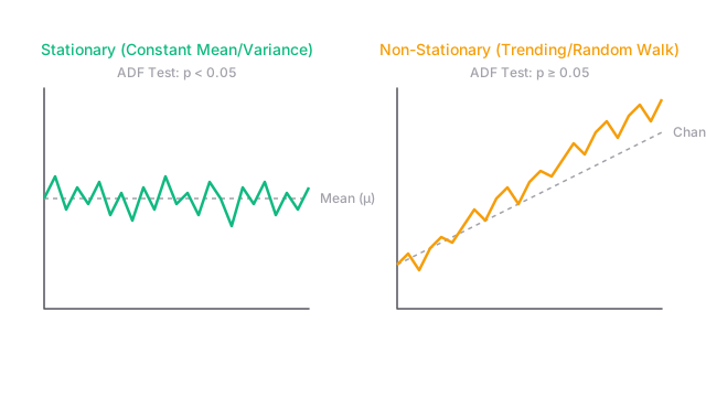
ARIMA, VAR, and most classical time series models assume the series is stationary — that the mean and variance don't change over time. Fitting these models to a non-stationary series (one with a trend or explosive variance) produces unreliable, often completely wrong estimates.

The Augmented Dickey-Fuller (ADF) and KPSS tests provide formal statistical procedures to decide whether a series needs to be transformed (via differencing or log transformation) before modeling.

Think of It Like This

Testing whether a car is level before aligning the wheels

Wheel alignment assumes the car is on a level surface. If the floor is tilted, the measurements are meaningless. Similarly, time series models assume the series is stationary. Testing for stationarity is checking whether the statistical "floor" is level before running any analysis on top of it.

How It Actually Works

What stationarity means

A strictly stationary series has the same joint distribution for any lag — all statistical properties are time-invariant. In practice, we use the weaker weak (covariance) stationarity:

Constant mean: $\mathbb{E}[y_t] = \mu \quad \forall t$
Constant variance: $\text{Var}(y_t) = \sigma^2 \quad \forall t$
Autocovariance depends only on lag: $\text{Cov}(y_t, y_{t-k}) = \gamma_k \quad \forall t$

A trending series violates condition 1. A series with increasing volatility violates condition 2.

Augmented Dickey-Fuller (ADF) test

The ADF test is the most widely used stationarity test. It tests for a unit root — the formal cause of non-stationarity in most financial and economic series.

Null hypothesis ( $H_0$ ): The series has a unit root (is non-stationary).
Alternative ( $H_1$ ): The series is stationary.

The test regresses $\Delta y_t = \alpha + \beta t + \gamma y_{t-1} + \sum_{i=1}^{p} \delta_i \Delta y_{t-i} + \varepsilon_t$ and tests $H_0: \gamma = 0$ .

Interpretation:

p-value < 0.05: Reject $H_0$ → series is stationary (no unit root)
p-value ≥ 0.05: Fail to reject $H_0$ → series likely has a unit root (non-stationary)

KPSS test (complementary)

The KPSS test reverses the null and alternative:

Null hypothesis ( $H_0$ ): The series IS stationary.
Alternative ( $H_1$ ): The series has a unit root.

Used alongside ADF to distinguish "has a unit root" from "trend-stationary":

ADF result	KPSS result	Conclusion
Reject $H_0$	Fail to reject $H_0$	Stationary ✓
Fail to reject $H_0$	Reject $H_0$	Unit root (difference to fix)
Fail to reject $H_0$	Fail to reject $H_0$	Trend-stationary (detrend to fix)
Reject $H_0$	Reject $H_0$	Insufficient data / structural break

Making a series stationary

Problem	Transformation
Linear trend	First difference: $\Delta y_t = y_t - y_{t-1}$
Exponential trend	Log then first difference: $\Delta \log y_t$
Seasonal non-stationarity	Seasonal difference: $\Delta_m y_t = y_t - y_{t-m}$
Increasing variance	Log or Box-Cox transform

The order of integration $I(d)$ is the number of differences needed to achieve stationarity. $I(0)$ = already stationary; $I(1)$ = needs 1 difference (most economic series); $I(2)$ = needs 2 differences (rare).

Code

1import numpy as np2import pandas as pd3from statsmodels.tsa.stattools import adfuller, kpss4
5# ── Generate non-stationary and stationary series ─────────────────────────────6np.random.seed(42)7n = 2008
9# Non-stationary: random walk (unit root)10y_nonstat = np.cumsum(np.random.randn(n))11
12# Stationary: mean-reverting AR(1) with |φ| < 113y_stat = np.zeros(n)14for t in range(1, n):15    y_stat[t] = 0.7 * y_stat[t-1] + np.random.randn()16
17
18def run_stationarity_tests(series, name):19    print(f"\n{'='*50}")20    print(f"Series: {name}")21    print(f"Mean: {series.mean():.3f}, Std: {series.std():.3f}")22    23    # ── ADF test ──────────────────────────────────────────────────────────────24    adf_result = adfuller(series, autolag='AIC')25    print(f"\nADF Test:")26    print(f"  Test statistic: {adf_result[0]:.4f}")27    print(f"  p-value:        {adf_result[1]:.4f}")28    print(f"  Lags used:      {adf_result[2]}")29    print(f"  Critical values: 1%={adf_result[4]['1%']:.3f}  "30          f"5%={adf_result[4]['5%']:.3f}  10%={adf_result[4]['10%']:.3f}")31    adf_conclusion = "STATIONARY" if adf_result[1] < 0.05 else "NON-STATIONARY (unit root)"32    print(f"  Conclusion: {adf_conclusion}")33    34    # ── KPSS test ─────────────────────────────────────────────────────────────35    kpss_result = kpss(series, regression='c', nlags='auto')36    print(f"\nKPSS Test:")37    print(f"  Test statistic: {kpss_result[0]:.4f}")38    print(f"  p-value:        {kpss_result[1]:.4f}")39    kpss_conclusion = "NON-STATIONARY" if kpss_result[1] < 0.05 else "STATIONARY"40    print(f"  Conclusion: {kpss_conclusion}")41    42    # ── Differencing if needed ────────────────────────────────────────────────43    if adf_result[1] >= 0.05:44        series_diff = np.diff(series)45        adf_diff = adfuller(series_diff, autolag='AIC')46        print(f"\nAfter 1st differencing:")47        print(f"  ADF p-value: {adf_diff[1]:.4f} → "48              f"{'STATIONARY ✓' if adf_diff[1] < 0.05 else 'still non-stationary'}")49
50
51run_stationarity_tests(y_nonstat, "Random Walk (non-stationary)")52run_stationarity_tests(y_stat,    "AR(1) φ=0.7 (stationary)")53
54# ── Real-world example: test then difference ──────────────────────────────────55print("\n--- ADF decision function ---")56def ensure_stationary(series, max_diffs=3):57    """Difference until stationary, return transformed series and order."""58    for d in range(max_diffs + 1):59        result = adfuller(series, autolag='AIC')60        if result[1] < 0.05:61            print(f"  Stationary at d={d} (p={result[1]:.4f})")62            return series, d63        print(f"  d={d}: p={result[1]:.4f} → applying difference")64        series = np.diff(series)65    print("  WARNING: could not achieve stationarity in {max_diffs} differences")66    return series, max_diffs67
68_, integration_order = ensure_stationary(y_nonstat)

Watch Out For

Conflating stationarity tests with certainty

ADF and KPSS are hypothesis tests with Type I and Type II errors. For short series (< 100 observations), both tests have low power — they may fail to detect non-stationarity even when it's present. Supplement formal tests with visual inspection of rolling mean and variance, and with the ACF correlogram.

Over-differencing

Differencing once too many times (applying $\Delta$ to an already-stationary series) introduces spurious moving-average components and makes the series harder to model. Use the minimum number of differences needed to pass the ADF test. If ADF already rejects $H_0$ at $d=0$ , the series is already stationary — do not difference.

The Quick Version

Stationarity = constant mean, variance, and autocovariance structure over time.
ADF test: $H_0$ = unit root (non-stationary); reject $H_0$ (p < 0.05) → stationary.
KPSS test: $H_0$ = stationary; reject $H_0$ (p < 0.05) → non-stationary.
Use both tests together — they help distinguish unit-root non-stationarity from trend-stationarity.
Transform to achieve stationarity: first difference for linear trends, log for exponential growth, seasonal difference for seasonal patterns.