Time Series Fundamentals

A time series is a sequence of observations indexed by time — and forecasting it requires understanding the patterns hidden in that sequence: trends, seasonality, cycles, and noise, each requiring different modeling approaches.

Why Does This Exist?

Time-ordered data requires different treatment than cross-sectional data. Standard ML assumes i.i.d. (independent and identically distributed) samples. Time series observations violate this: tomorrow's temperature depends on today's; next quarter's sales depend on last quarter's patterns. Applying standard ML without accounting for temporal dependencies produces models that appear accurate but fail in deployment.

Time series problems appear everywhere: demand forecasting for supply chains, energy consumption prediction, financial price prediction, patient vitals monitoring, network traffic anomaly detection.

Think of It Like This

A detective reading the history of a city

A time series is like reading a city's history: some patterns are long-term trends (population grew steadily from 1950 to 2020), some are seasonal (crime spikes in summer), some are cyclical (economic booms and busts every 7–10 years), and some are random events (a pandemic in 2020). A forecaster, like a detective, reads these overlapping patterns and extrapolates what comes next — while knowing that truly random events cannot be predicted.

How It Actually Works

The four components

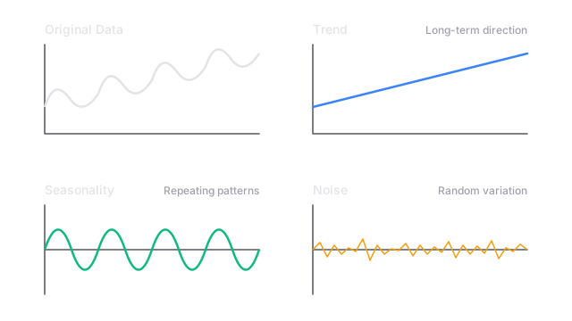
A time series $y_t$ can be decomposed into:

$y_t = T_t + S_t + C_t + \varepsilon_t$

Component	Symbol	Description
Trend	$T_t$	Long-run direction (up, down, flat)
Seasonality	$S_t$	Periodic fluctuations with fixed period (weekly, annual)
Cycles	$C_t$	Irregular long-term oscillations (business cycles)
Noise	$\varepsilon_t$	Random, unpredictable variation

Alternatively, if the pattern amplifies over time (seasonal swings grow with the trend), use multiplicative decomposition: $y_t = T_t \times S_t \times C_t \times \varepsilon_t$ .

Autocorrelation

The key statistical property that distinguishes time series: observations at time $t$ are correlated with observations at time $t-k$ (lag $k$ ).

Autocorrelation function (ACF): $\rho_k = \text{Corr}(y_t, y_{t-k})$

If sales this week correlate with sales last week: $\rho_1 > 0$ . If there's a weekly pattern, $\rho_7$ will be high. Plotting the ACF for all lags gives the correlogram, the first diagnostic tool for any time series.

Stationarity

A stationary time series has constant statistical properties over time: constant mean, constant variance, and ACF depending only on lag, not on time position.

$\mathbb{E}[y_t] = \mu \quad \forall t \qquad \text{Var}(y_t) = \sigma^2 \quad \forall t$

Most forecasting models require stationarity. Non-stationary series (with trends or changing variance) must be transformed:

Differencing removes trends: $\Delta y_t = y_t - y_{t-1}$
Log transformation stabilizes variance: $\tilde{y}_t = \log(y_t)$
Seasonal differencing removes seasonality: $\Delta_{12} y_t = y_t - y_{t-12}$

Code

1import pandas as pd2import numpy as np3import matplotlib4matplotlib.use('Agg')  # non-interactive backend5
6# ── Generate synthetic time series ────────────────────────────────────────────7np.random.seed(42)8dates = pd.date_range("2020-01-01", periods=104, freq="W")9
10trend      = np.linspace(100, 200, 104)11seasonality = 20 * np.sin(2 * np.pi * np.arange(104) / 52)12noise      = np.random.normal(0, 5, 104)13y = trend + seasonality + noise14
15ts = pd.Series(y, index=dates, name="weekly_sales")16
17# ── Basic statistics ──────────────────────────────────────────────────────────18print("Time series summary:")19print(f"  Length: {len(ts)} weeks")20print(f"  Mean:   {ts.mean():.2f}")21print(f"  Std:    {ts.std():.2f}")22print(f"  Range:  [{ts.min():.2f}, {ts.max():.2f}]")23
24# ── Autocorrelation function ──────────────────────────────────────────────────25from statsmodels.stats.stattools import durbin_watson26from pandas.plotting import autocorrelation_plot27
28# Manual ACF computation29def acf_values(series, max_lag=20):30    acf = [1.0]  # lag 031    for k in range(1, max_lag + 1):32        corr = np.corrcoef(series[k:], series[:-k])[0, 1]33        acf.append(corr)34    return acf35
36acf = acf_values(ts.values)37print("\nACF values:")38for lag, val in enumerate(acf[:10]):39    print(f"  Lag {lag:>2}: {val:+.3f}")40
41# ── Classical decomposition ───────────────────────────────────────────────────42from statsmodels.tsa.seasonal import seasonal_decompose43
44decomposition = seasonal_decompose(ts, model='additive', period=52)45print("\nDecomposition components:")46print(f"  Trend range:       [{decomposition.trend.dropna().min():.1f}, {decomposition.trend.dropna().max():.1f}]")47print(f"  Seasonal range:    [{decomposition.seasonal.min():.1f}, {decomposition.seasonal.max():.1f}]")48print(f"  Residual std:      {decomposition.resid.dropna().std():.2f}")49
50# ── Differencing to achieve stationarity ─────────────────────────────────────51ts_diff = ts.diff().dropna()52print(f"\nAfter first differencing:")53print(f"  Mean: {ts_diff.mean():.4f} (≈0 → trend removed)")54print(f"  Std:  {ts_diff.std():.2f}")

Watch Out For

Data leakage in train-test splits

With time series, you cannot randomly shuffle and split — the test set must be strictly after the training set in time. Using a random split leaks future information into training (the model sees data from "the future" during training), producing unrealistically optimistic metrics. Always split chronologically.

Assuming stationarity without testing

Many forecasting models (ARIMA, linear regression) assume stationarity. Applying them to a non-stationary series (trending, heteroskedastic) produces unreliable estimates. Always test stationarity (Augmented Dickey-Fuller or KPSS test) and apply the appropriate transformation before fitting.

The Quick Version

A time series is observations indexed by time — observations are not i.i.d.; they have temporal dependencies.
Four components: trend (long-run direction), seasonality (periodic pattern), cycles (irregular oscillations), noise.
Autocorrelation measures the correlation between a series and its own lagged values — the fundamental diagnostic.
Stationarity (constant mean and variance over time) is required by most classical forecasting models.
Transform non-stationary series: differencing removes trends, log transformation stabilizes variance.