Flow Matching

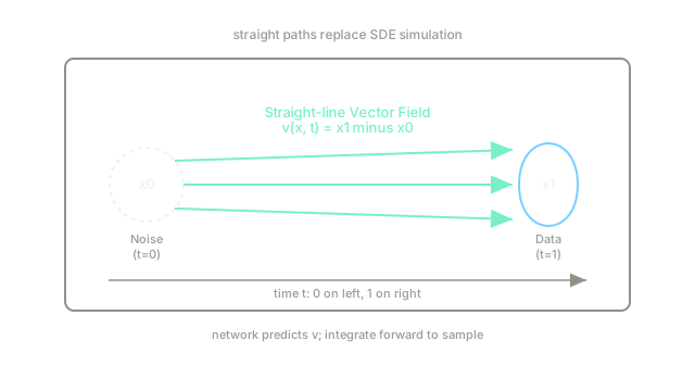
The Problem

Score-based diffusion models (using Stochastic Differential Equations) were mathematically elegant but difficult to train and simulate. Calculating the "score function" required simulating a complex forward diffusion process, which was slow and mathematically constrained. Researchers wanted a simpler way to map a simple distribution (noise) to a complex one (images) without the baggage of Markov chains or Brownian motion.

The Idea

Meta AI researchers introduced Flow Matching. Instead of relying on diffusion processes, they viewed generation as a Continuous Normalizing Flow (CNF). The goal is simply to construct a "vector field"—a set of arrows showing how probability mass should flow from a noise distribution to a data distribution. Flow Matching proves that you don't need to simulate complex paths; you can simply draw straight lines between random noise points and random images, and train a neural network to predict the direction (the vector) of those lines.

How It Works

The framework drastically simplifies the math:

1. The Vector Field: At time $t=0$, you have pure noise $x_0$. At time $t=1$, you have a real image $x_1$. The easiest path between them is a straight line: $x_t = (1-t)x_0 + t x_1$.
2. The Target: The derivative (velocity) of this straight line is simply $x_1 - x_0$. This is the "vector field" the network needs to learn.
3. Training (Flow Matching): A neural network is trained to predict this velocity vector given $x_t$ and $t$. The loss is a simple Mean Squared Error between the network's prediction and the true straight-line velocity.
4. Generation: To generate, you sample noise $x_0$, and use an ODE solver to follow the velocity field predicted by the network until $t=1$.

Why It Mattered

Flow Matching (specifically Optimal Transport Flow Matching) provided a strictly simpler, faster, and more general alternative to diffusion models. Because the trajectories are straight lines (unlike the curved, noisy trajectories of diffusion SDEs), the ODE solvers can take much larger steps during generation, leading to faster sampling with fewer steps.

What Came After

Flow Matching rapidly gained traction as the successor to standard diffusion. It is the underlying mathematical framework for Stable Diffusion 3, replacing the older DDPM/SDE frameworks. It also proved highly effective for scientific applications, like modeling protein dynamics.