Semi-Supervised Classification with Graph Convolutional Networks

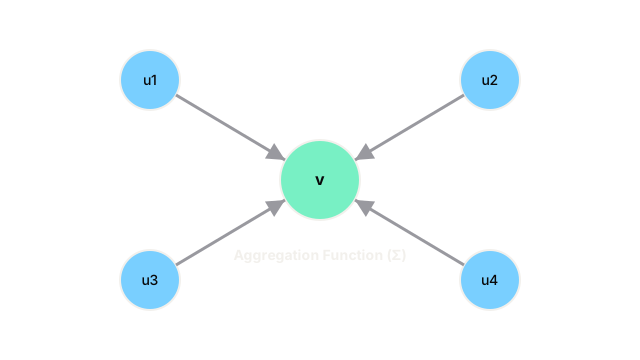
The Problem

Many real-world datasets naturally exist as graphs, such as social networks, citation networks, and molecular structures. Traditional neural networks (like CNNs or MLPs) expect grid-like data (images) or sequential data (text) and struggle to process graph-structured data effectively. Previous attempts to apply neural networks to graphs were either computationally expensive, lacked scalability, or failed to adequately capture both the node features and the graph topology simultaneously, particularly in semi-supervised settings where only a small fraction of nodes have labels.

The Idea

The authors proposed Graph Convolutional Networks (GCNs), an efficient and scalable method to perform convolution-like operations directly on graphs. The core idea is to update the representation of a node by aggregating the representations of its immediate neighbors, alongside its own features. By stacking multiple GCN layers, a node can incorporate information from its extended neighborhood, learning powerful localized representations driven by both the node features and the underlying graph structure.

How It Works

The GCN model simplifies prior graph convolutions by using a first-order approximation of spectral graph convolutions. The layer-wise propagation rule is defined as:

1. Self-Loops: The adjacency matrix $A$ of the graph is modified to include self-loops ($\tilde{A} = A + I$), ensuring that a node's own features are considered during aggregation.
2. Normalization: The modified adjacency matrix is symmetrically normalized using the degree matrix ($\tilde{D}^{-\frac{1}{2}} \tilde{A} \tilde{D}^{-\frac{1}{2}}$) to prevent features from scaling up with the number of connections.
3. Feature Transformation: The normalized adjacency matrix is multiplied by the node feature matrix $H^{(l)}$ from the previous layer, and then transformed by a learnable weight matrix $W^{(l)}$.
4. Non-linearity: An activation function (like ReLU) is applied.

The full equation for a layer is: $H^{(l+1)} = \sigma \left( \tilde{D}^{-\frac{1}{2}} \tilde{A} \tilde{D}^{-\frac{1}{2}} H^{(l)} W^{(l)} \right)$. This operation essentially acts as a localized message-passing mechanism where nodes average the features of their neighbors and themselves.

Why It Mattered

GCNs offered a massive leap forward in Graph Neural Networks by dramatically simplifying the convolution operation on graphs while improving performance. They were highly scalable and achieved state-of-the-art results on standard graph benchmarks (like Cora, Citeseer, and Pubmed) for semi-supervised node classification. GCNs provided a clear, intuitive framework (message passing) that bridged the gap between deep learning and graph theory, making GNNs accessible to a wider range of researchers and practitioners.

What Came After

The GCN paper ignited an explosion of research in Graph Neural Networks. It paved the way for numerous extensions, including Graph Attention Networks (GAT) which introduced attention mechanisms to weigh neighbor contributions differently, and GraphSAGE, which enabled inductive learning on large, dynamic graphs. GCNs are now foundational models, applied in diverse domains ranging from drug discovery and traffic prediction to recommendation systems and fraud detection.