Vanilla RNN

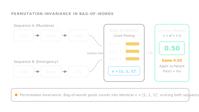
Traditional bag-of-words (BoW) models discard sequence ordering by pooling token counts into a static frequency histogram. When meaning depends entirely on word order, permutation invariance breaks comprehension:

• Permutation invariance: Consider two phrases with opposite meanings: "dog bites man" (mundane event) versus "man bites dog" (sensational news). In a three-word vocabulary $\mathcal{V} = \{\text{dog}, \text{bites}, \text{man}\}$, both sentences map to the identical multiset count vector: $v_A = v_B = \begin{bmatrix} 1 \\ 1 \\ 1 \end{bmatrix}$
• The agency void: Because the representation is identical ($f(\pi(x)) = f(x)$), any linear classifier $s = \sigma(w^T v + b)$ outputs the exact same prediction score ($0.50$) for both inputs. A bag of words cannot determine grammatical roles, agent-patient relationships, or temporal causality. Language requires directional sequence processing.

Read, Note, Carry On

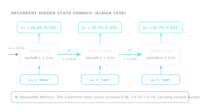
The Recurrent Neural Network (Elman, 1990) processes sentences sequentially from left to right, maintaining a dynamic hidden state vector $h_t$ that carries forward an accumulated memory summary:

• The state update equation: At each time step $t$, the recurrent cell combines the new token input vector $x_t$ with the preceding hidden state $h_{t-1}$: $h_t = \tanh(W x_t + U h_{t-1} + b)$ where $W$ weights the incoming token and $U$ governs the recurrent transition.
• Tracking context forward: Reading "the cat sat" with initial resting state $h_0 = [0.00, 0.00]^T$:
  1. Step 1 ("the"): Ingests the determiner, initializing the context vector to $h_1 = [0.46, 0.20]^T$.
  2. Step 2 ("cat"): Fuses subject semantics into the running note, advancing memory to $h_2 = [0.70, 0.45]^T$.
  3. Step 3 ("sat"): Incorporates the action verb, yielding $h_3 = [0.79, 0.62]^T$. Every step updates the same compact memory vector, preserving the trajectory of preceding tokens.

One Cell, Every Step

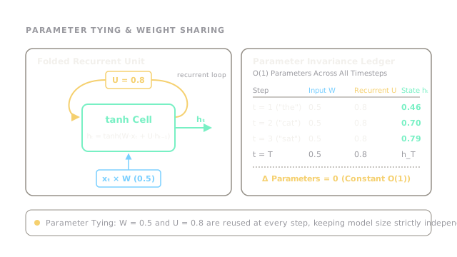
The core design principle of recurrent architectures is parameter tying across time:

• Shared weight matrices: Rather than instantiating unique parameters for each word index, a single recurrent unit reuses the identical weight matrices $W = 0.5$ and $U = 0.8$ across every time step: $h_t = \tanh(0.5 x_t + 0.8 h_{t-1} + b)$
• Constant parameter footprint: Because the same cell loops indefinitely, total model parameters remain strictly $\mathcal{O}(1)$. Whether processing a five-word headline or a thousand-word transcript, no new parameters are allocated ($\Delta P = 0$). Parameter sharing enforces temporal translation equivariance across the sequence.

Same Cell Any Length

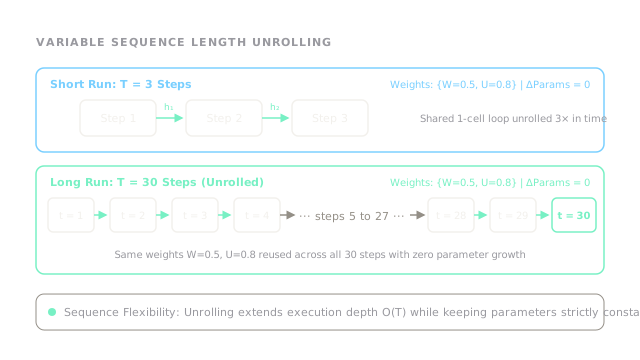
Feedforward architectures like Multi-Layer Perceptrons require fixed input dimensionalities ($X \in \mathbb{R}^{d_{\text{in}}}$), requiring padding, truncating, or exploding parameter counts for long sequences. Recurrent networks unroll dynamically:

• Dynamic unrolling: An RNN handles arbitrary sequence length $T \in [1, \infty)$ by unrolling through time.
• Short versus long runs: A three-step phrase ($T = 3$) and an unrolled thirty-step paragraph ($T = 30$) execute through the exact same two weight matrices ($W = 0.5$, $U = 0.8$). Sequence length changes only the depth of the computational graph during forward execution, never the parameter capacity of the model.

Yesterday Whispers, Then Hushes

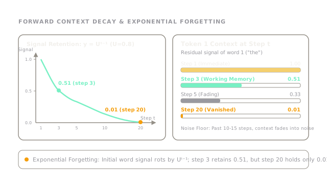
While recurrent parameter sharing allows processing arbitrary lengths, vanilla RNNs suffer from forward information decay:

• Exponential signal decay: The contribution of the initial token $x_1$ to the hidden state at step $t$ decays roughly as the power of the recurrent transition weight: $\frac{\partial h_t}{\partial h_1} \approx U^{t-1} \prod_{k=2}^t \text{diag}(1 - h_k^2)$
• Vanishing context horizon: For transition weight $U = 0.80$:
  • Step 1: $0.80^0 = 1.000$ ($100\%$ influence).
  • Step 3: $0.80^2 = 0.64 \implies 0.510$ ($51\%$ retention through $\tanh$ saturation).
  • Step 5: $0.80^4 \approx 0.330$ ($33\%$ retention).
  • Step 20: $0.80^{19} \approx 0.010$ ($1\%$ residual signal). By step twenty, the influence of early subject modifiers has drowned in noise, making vanilla RNNs unable to connect subject-verb dependencies across long clauses.

How Far Must Memory Reach?

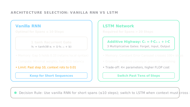
Selecting between a vanilla RNN and gated alternatives depends on the maximum dependency distance required by the task:

• Vanilla RNN (Short spans, $T \le 10$): Features a single $\tanh$ activation gate with simple $O(1)$ arithmetic. For local tasks like part-of-speech tagging or short sensor streams where dependency gaps rarely exceed five steps (retaining $0.33$ signal), vanilla RNNs provide fast, lightweight inference.
• LSTM (Long spans, $T > 20$): Long Short-Term Memory networks introduce three multiplicative gates (forget $f_t$, input $i_t$, output $o_t$) alongside an additive cell state conveyor belt: $C_t = f_t \odot C_{t-1} + i_t \odot \tilde{C}_t$ Because gradients can flow unattenuated along the additive cell highway ($\partial C_t / \partial C_{t-1} \approx 1$), LSTMs bridge dependencies exceeding 100 steps, justifying their $4\times$ parameter and compute overhead.

Where It Breaks

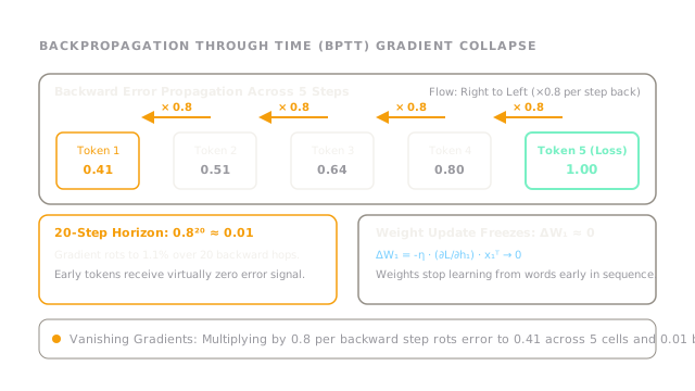
The fatal limitation of the vanilla RNN emerges during training via Backpropagation Through Time (BPTT):

• The backward chain rule: To update input weights $W$ based on an error loss $\mathcal{L}$ at terminal step $T$, error gradients must backpropagate through the entire recurrent chain: $\frac{\partial \mathcal{L}}{\partial h_1} = \frac{\partial \mathcal{L}}{\partial h_T} \prod_{t=2}^T \frac{\partial h_t}{\partial h_{t-1}} = \frac{\partial \mathcal{L}}{\partial h_T} \prod_{t=2}^T \text{diag}(1 - h_t^2) U^T$
• Vanishing gradients: Because $|\tanh'(z)| \le 1.0$ and $|U| = 0.80 < 1.0$, every backward step multiplies the error signal by a factor $\le 0.80$:
  • Step 5 (Loss origin): Error signal $= 1.00$.
  • Step 4: $1.00 \times 0.80 = 0.80$.
  • Step 3: $0.80 \times 0.80 = 0.64$.
  • Step 1: $0.51 \times 0.80 = 0.41$.
  • Step 20 (Long sequence): $0.80^{20} \approx 0.011 \approx 0.01$.
• Learning paralysis: With gradients attenuated to $0.01$, weight updates for early tokens ($\Delta W_1 = -\eta \frac{\partial \mathcal{L}}{\partial h_1} x_1^T$) freeze completely. The network optimizes only for immediate, local token transitions while remaining permanently blind to long-range syntactic structure.

The Quick Version

• Bag of words pools frequencies, predicting the same score ($0.50$) for "dog bites man" and "man bites dog".
• Elman RNNs maintain a 2-number hidden state summary that advances from $0.46$ to $0.79$ across tokens.
• Parameter sharing reuses input weight $W=0.5$ and recurrent weight $U=0.8$ across all steps with $O(1)$ memory.
• Dynamic unrolling processes three steps or thirty using the exact same cell without allocating new weights.
• Context decays exponentially as $U^{t-1}$: step 3 preserves $0.51$ context, while step 20 retains only $0.01$.
• Choose vanilla RNNs for cheap short spans ($\le 10$ steps); upgrade to gated LSTMs for long spans ($>20$ steps).
• Backpropagation multiplies gradients by $\le 0.80$ per step, decaying error to $0.01$ and freezing early token learning.