Visual explainer
Variational Autoencoders
Trace Gaussian latent codes, reparameterized sampling and the reconstruction–KL objective, then see why prior sampling can still fail.
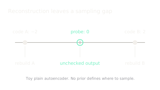
A plain autoencoder learns to rebuild inputs from their codes. That objective does not define a probability distribution for drawing new codes or guarantee useful outputs between them. A variational autoencoder adds a generative model with a latent prior and learns an approximate posterior for each input.
Predict A Gaussian Posterior
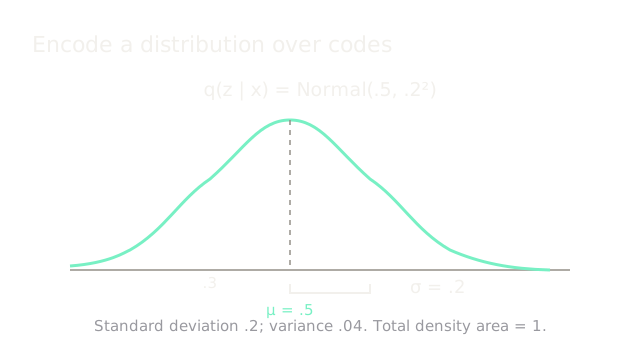
In the common diagonal-Gaussian VAE, the encoder predicts a mean and variance for each latent dimension, often parameterizing the log variance. Our one-dimensional example has mean .5 and standard deviation .2, so variance is .04. This distribution approximates p(z | x); it is not a guaranteed safe decoding region.
Sample With Real Numbers
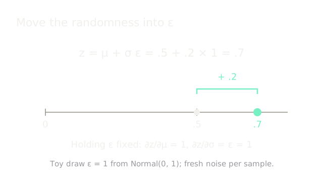
Draw ε from a standard normal, then compute z = μ + σε. For the illustrative draw ε=1, .5 + .2 × 1 = .7. Holding the draw fixed gives derivatives ∂z/∂μ=1 and ∂z/∂σ=1, allowing reconstruction gradients to reach the encoder parameters.
Penalize Departure From Prior
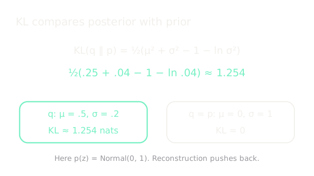
With prior p(z)=Normal(0,1), the analytic KL term is ½(μ²+σ²−1−ln σ²). Our posterior costs about 1.254 nats. This regularizer competes with reconstruction, encouraging compatibility with the prior without guaranteeing that all latent locations become useful.
Generate From The Prior
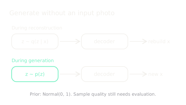
Reconstruction samples from the input-conditioned encoder distribution. Generation instead draws z from the prior and passes it to the same learned decoder, which defines p(x | z). No input photo is needed. Held-out reconstruction and prior-sample quality need separate evaluation.
Tune The KL Weight
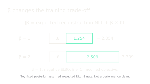
The standard negative evidence lower bound (ELBO) is expected reconstruction negative log-likelihood plus KL. A β-weighted variant changes the latter's weight. Holding our posterior fixed and assuming reconstruction cost .8 nats gives totals 2.054 at β=1 and 3.309 at β=2. Retraining changes both terms; β does not guarantee sharpness or smoothness.
Where It Breaks
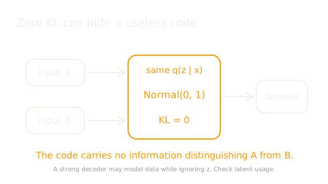
A strong decoder may ignore the latent variable while the encoder matches the prior for every input. Then KL approaches zero without an informative code. This posterior-collapse failure requires checking latent usage alongside likelihood and samples. Blurry image reconstructions are another possible limit, influenced by the likelihood model and decoder rather than an unavoidable consequence of sampling.
The Quick Version
- Reconstruction alone does not define a latent sampling distribution.
- Gaussian encoders predict means and positive standard deviations.
- Mean .5 plus .2 times noise 1 gives .7.
- KL regularizes the posterior toward a chosen prior.
- Generation samples the prior, then uses the decoder.
- Beta weights KL against expected reconstruction cost.
- Zero KL can accompany an uninformative latent representation.