Jacobians and Singularities

An arm can reach a point yet struggle to move through it in a particular direction. The Jacobian maps joint speeds to the tip's instantaneous velocity; a singularity is a posture where that map loses rank relative to its attainable maximum. The lost direction depends on the task you ask the robot to perform.

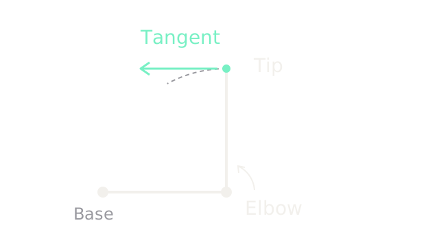
Start with a synthetic planar arm: two one-metre links, shoulder angle $q_1=0$, elbow angle $q_2=90^\circ$, and tip position $(1,1)$ metres. The shoulder angle is counterclockwise from world x; the elbow angle is relative to the first link. World y points up. The elbow pivots at $(1,0)$, so its tip initially moves left when the elbow turns counterclockwise. The dashed arc shows the curved path; the straight arrow shows its tangent, not a finite displacement.

This page studies two-dimensional tip position, with joint angles in radians for derivatives. It does not constrain tool orientation. Forward and inverse kinematics covers where the tip is; here we ask how fast it can move. Arm scenes use 180 drawing units per metre until a zoom is stated.

One column per joint

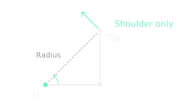
Freeze the elbow coordinate and turn only the shoulder. The whole bent arm rotates about the base. Its tip velocity is perpendicular to the dashed base-to-tip radius, which is $(1,1)$ m. A positive unit shoulder rate therefore contributes $(-1,1)$ m/s: left and up.

That vector is the Jacobian's first column. A column answers: what tip velocity would one unit of this joint's rate produce, with the other joint rates zero? The picture uses an actual shoulder rate of $0.5$ rad/s, giving $(-0.5,0.5)$ m/s. Velocity arrows use 120 drawing units per m/s, a separate scale from the arm. The small joint arc identifies the rotation direction.

Find the elbow column

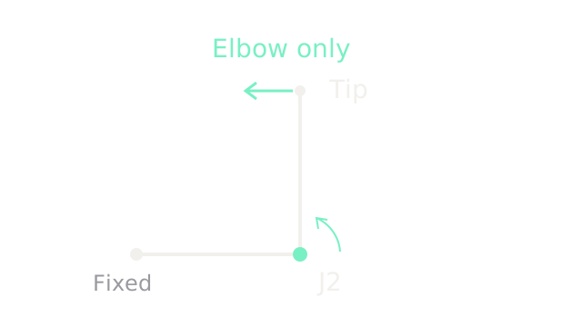
Hold the shoulder still. The tip rotates about the elbow, rather than the base. Its radius is now $(0,1)$ m, so a unit elbow rate contributes $(-1,0)$ m/s. At $0.5$ rad/s, the tip velocity is $(-0.5,0)$ m/s. The same velocity scale makes this arrow shorter than the shoulder contribution.

Collect the two columns, with the x component above the y component:

$$J(q)=\frac{\partial(x,y)}{\partial(q_1,q_2)},\qquad J(0,\pi/2)=\begin{bmatrix}-1&-1\\1&0\end{bmatrix}\ \mathrm{m/rad}.$$

The derivative comes from differentiating $x=\cos q_1+\cos(q_1+q_2)$ and $y=\sin q_1+\sin(q_1+q_2)$ for our one-metre links. The Jacobian depends on posture: a column that points left here can point somewhere else after the arm moves.

Add the contributions

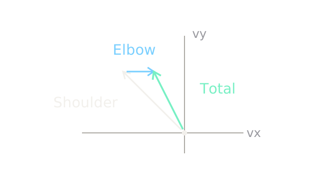
The diagram now shows velocity space, not another arm posture. Axes are $v_x$ and $v_y$, and arrows use 600 drawing units per m/s. Set shoulder rate $\dot q_1=0.2$ rad/s and elbow rate $\dot q_2=-0.1$ rad/s. Multiply each column by its joint rate:

$$v_1=(-0.2,0.2),\qquad v_2=(0.1,0),\qquad \dot p=J\dot q=v_1+v_2=(-0.1,0.2)\ \mathrm{m/s}.$$

Here $\dot q$ collects the joint rates, and $\dot p$ is tip velocity. The blue elbow arrow starts at the shoulder arrow's head; the mint resultant joins the common origin to the final head. Negative elbow rotation cancels part of the leftward motion without changing the upward component. Joint rates are not the tip's x and y speeds.

Local is not global

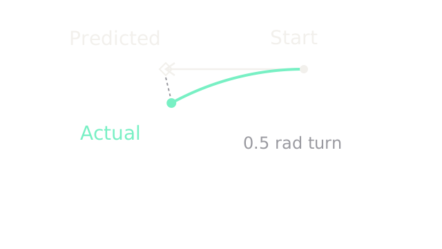
The velocity relation is exact at an instant for the ideal rigid model. Its finite-step version, $\Delta p\approx J(q)\Delta q$, is an approximation. Return to the starting posture, keep the shoulder fixed, and turn the elbow by $0.5$ rad. A frozen Jacobian predicts

$$p_{\mathrm{linear}}=(1,1)+(-1,0)\,0.5=(0.5,1)\ \mathrm{m}.$$

Forward kinematics instead gives $p_{\mathrm{actual}}=(1-\sin0.5,\cos0.5)\approx(0.520574,0.877583)$ m. The error is approximately $(0.020574,-0.122417)$ m. The detail view uses 400 drawing units per metre: the diamond is the tangent prediction and the mint dot is the actual endpoint. The elbow lies below the cropped view; the mint path is a circular arc of radius one metre.

Use smaller steps and recompute the Jacobian as posture changes. A single local inverse is not a global inverse-kinematics solution or a collision-free trajectory.

Solve the inverse rate problem

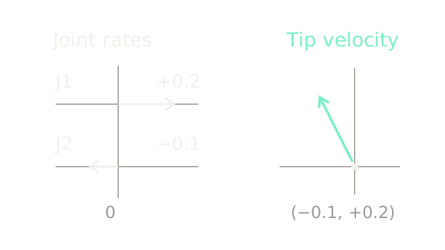
Suppose you command $\dot p=(-0.1,0.2)$ m/s at the original posture. Solve the two rows of $J\dot q=\dot p$:

$$-\dot q_1-\dot q_2=-0.1,\qquad \dot q_1=0.2.$$

The second row fixes the shoulder rate at $0.2$ rad/s. Substituting into the first gives $\dot q_2=-0.1$ rad/s, recovering our earlier example. The left bars share a zero and use 400 drawing units per rad/s; the right vector uses 500 per m/s.

This square matrix is invertible because its determinant is one. A robot with more joints than task coordinates can have multiple rate solutions; a robot with fewer independent task directions cannot realize every request. A matrix's dimensions alone do not tell you its rank at the current posture.

See the velocity ellipse

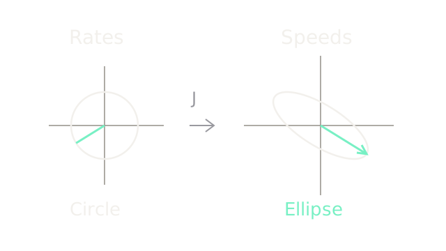
Consider every joint-rate pair with $\sqrt{\dot q_1^2+\dot q_2^2}=0.2$ rad/s. Those pairs form the left circle. Apply $J$ to each pair and the tip velocities form the right manipulability ellipse. The highlighted radius maps to the highlighted longest output radius; it is not an arbitrary matching colour.

For our matrix, $JJ^\mathsf{T}=[[2,-1],[-1,1]]$. Its eigenvalues are $(3\pm\sqrt5)/2$, so the singular values of $J$ are approximately $1.618034$ and $0.618034$ m/rad. Multiplying by $0.2$ gives ellipse semiaxes $0.323607$ and $0.123607$ m/s. Both plots use 240 drawing units per respective unit; joint-rate and tip-velocity units differ. The long axis is tilted about $31.7^\circ$ clockwise on screen because world y points up.

The ratio of the semiaxes is about $2.618$: equal joint-rate norms produce different attainable speeds in different directions. This circle assumes a joint-rate norm budget. Independent actuator speed bounds instead form a box in joint-rate space, whose linear image is generally a polygon. The ellipse is not a literal torque or collision limit.

Near a singularity

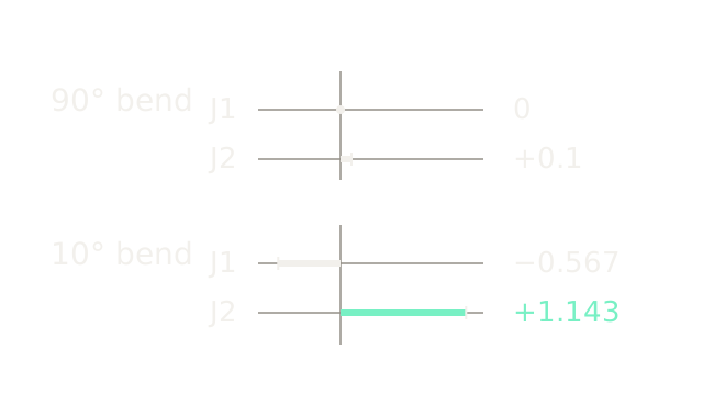
Keep $q_1=0$ and request the same leftward velocity $(-0.1,0)$ m/s. At $q_2=90^\circ$, the solution is $(0,0.1)$ rad/s. At $q_2=10^\circ$, the Jacobian becomes

$$J=\begin{bmatrix}-\sin10^\circ&-\sin10^\circ\\1+\cos10^\circ&\cos10^\circ\end{bmatrix}.$$

Solving gives $\dot q_1=-0.1\cot10^\circ\approx-0.567128$ and $\dot q_2=0.1(1+\cos10^\circ)/\sin10^\circ\approx1.143005$ rad/s. The signed bars share a scale of 100 drawing units per rad/s. Large opposing rates cancel vertical motion while creating the small leftward motion.

For these one-metre links, $\det J=\sin q_2$. As $q_2$ approaches zero, the weaker ellipse axis shrinks. Exact inversion can demand rates beyond the actuators' limits. Not every request becomes large: the poorly supported direction is the problem.

Respect the rate budget

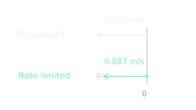
Assume each joint is limited to a magnitude of $1$ rad/s, an illustrative limit rather than a hardware specification. The elbow's requested $1.143005$ rad/s is too fast. Scale both rates by $\alpha=1/1.143005\approx0.874887$:

$$\dot q_{\mathrm{limited}}\approx(-0.496173,1),\qquad J\dot q_{\mathrm{limited}}=\alpha\dot p\approx(-0.087489,0)\ \mathrm{m/s}.$$

The lower arrow is shorter but still points left. The dashed extension marks the requested speed that was sacrificed. The two velocity arrows share 1600 drawing units per m/s. Scaling works because matrix multiplication is linear at a fixed posture; separately clipping one joint generally changes the tip direction.

This simple construction handles the stated speed bound only. Acceleration, torque, obstacles and tracking error need their own checks. Changing the path to avoid a weak posture can be more useful than insisting on the original speed.

Where it breaks

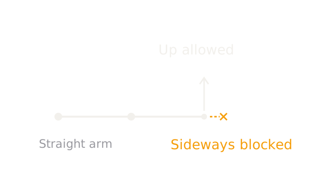
Fully straighten the arm: $q_1=q_2=0$, with the tip at $(2,0)$ m. This arm overview uses 150 drawing units per metre. Now

$$J=\begin{bmatrix}0&0\\2&1\end{bmatrix},\qquad \dot p=(0,\,2\dot q_1+\dot q_2).$$

Rank drops from two to one. The upward arrow is possible: $(\dot q_1,\dot q_2)=(0.08,0.04)$ rad/s gives $(0,0.2)$ m/s. A horizontal request of $(0.1,0)$ m/s has no solution for any finite joint rates. Velocity arrows use 400 drawing units per m/s; the cross stops the incompatible request.

For a combined request $(0.1,0.2)$ m/s, a minimum-norm pseudoinverse solution selects $(0.08,0.04)$ rad/s, realizing the vertical component and leaving horizontal residual $0.1$ m/s. A pseudoinverse or damped solver can choose manageable rates; it cannot create a missing direction. At this posture even inward horizontal velocity is unavailable to first order. Bending can later produce inward displacement through a curved path; outward displacement beyond the arm's maximum reach remains impossible.

The Quick Version

• Joint rotation moves the tip along a local tangent.
• Each Jacobian column describes one joint's instantaneous contribution.
• Different joints rotate the tip about different pivots.
• Weighted columns add to produce the tip velocity.
• Finite moves need updated Jacobians and forward checks.
• Inverse velocity kinematics solves rates for a requested tip velocity.
• A joint-rate circle maps to a velocity ellipse.
• Weak directions can demand large opposing joint rates.
• Uniform rate scaling preserves direction while reducing speed.
• Singularities remove instantaneous directions; numerical solvers cannot restore them.

Sources

Modern Robotics 5.3: Singularities develops Jacobian rank, joint-column contributions and unavailable task directions. Modern Robotics 5.4: Manipulability defines the velocity ellipsoid through a joint-rate sphere and the eigenstructure of $JJ^\mathsf{T}$. The arm, rate budget, numerical solutions and drawing scales above are explicitly synthetic calculations.