Model Predictive Control and Legged Locomotion

Model predictive control (MPC) repeatedly predicts how candidate actions will move a robot, optimizes a short future window, and applies the first action before planning again. For legged locomotion, those actions can be ground reaction forces at the stance feet. A useful plan must respect which feet touch the ground, available friction and the robot's ability to realize the requested forces.

Start with the ground

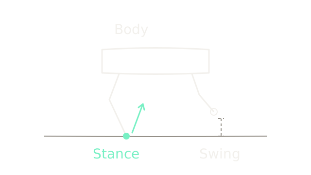
The solid dot is a planted stance foot; the ring is a swing foot above the surface. The gap beneath the ring matters: moving that leg does not create a ground reaction force there. The mint arrow represents the ground pushing back on the robot through the stance contact. Robot proportions in this opening sketch are schematic.

A motion plan can describe where the body should go. Locomotion control must find physically possible forces to move it there. A free-floating body cannot directly command its own position; it changes motion through external interactions. Joint motion can also redistribute orientation and angular momentum, so this is specifically a statement about ground force and overall linear momentum. See MIT's underactuation explanation.

Balance the body first

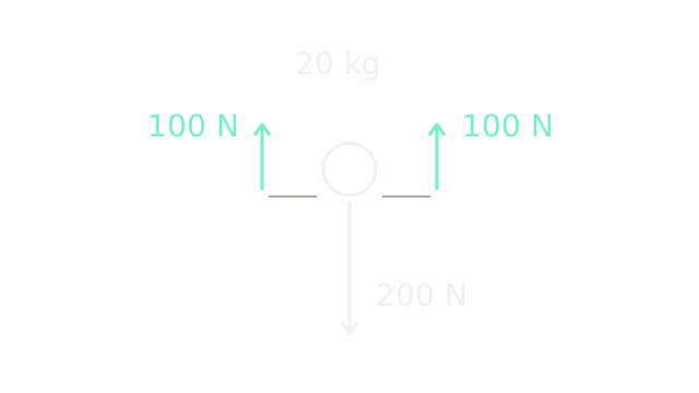
Replace the robot with a simplified body centered at its center of mass, the point representing its mass distribution for translational motion. The circle is that body; the separated upward arrows are its two support contributions, drawn apart for readability. Arrow length represents force at 0.6 drawing units per newton.

Our synthetic robot has mass $m=20$ kg. Use rounded teaching gravity $g=10$ m/s², giving weight $mg=200$ N. Two symmetric stance feet each provide 100 N upward:

$a_z=\frac{100+100}{20}-10=0.$

Here $a_z$ is vertical acceleration. Zero acceleration preserves the current vertical velocity; holding height also requires starting with zero vertical velocity. If each contact additionally supplies 20 N forward, the horizontal acceleration is $a_x=(20+20)/20=2$ m/s². The next beats use that forward motion. Equal total support alone does not establish rotational balance.

Decide which feet can push

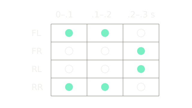
Read each column as one 0.1-second interval. FL and FR mean front left and front right; RL and RR mean rear left and rear right. Filled circles are stance, rings are swing. The first two intervals permit FL and RR to push; the third permits the other diagonal pair. This is a short crop, not a complete gait cycle.

In this formulation the schedule is an input to force optimization. For a swing leg, set its contact force to zero. For a stance leg, allow only admissible contact forces. Predicting continuous forces with a known contact sequence is a different problem from also choosing touchdown times and footholds. MIT's contact dynamics notes explain that distinction and the impact events between contact modes.

For the numerical example, track translation only and idealize the exchange of support. We omit moment balance, impact and leg inertia. Horizontal forces below the center of mass also create a pitch moment, so the upcoming rollout is not a full-body feasibility certificate. A real touchdown may change velocities and violate the smooth approximation.

Roll the model forward

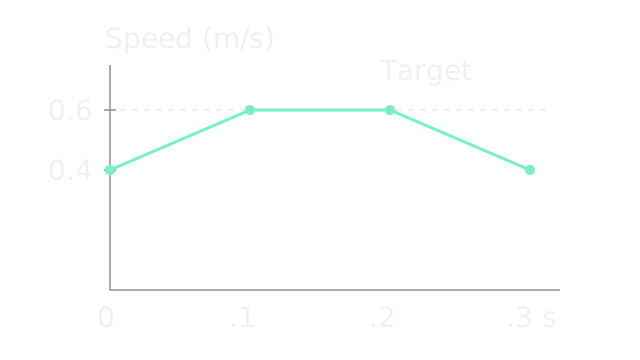
The horizontal axis is time; the vertical axis is forward speed, with a zero baseline. A dashed line marks the desired 0.6 m/s. The solid line is one candidate prediction. At constant acceleration $a_k$ during interval $k$, with interval length $\Delta t=0.1$ s:

$v_{k+1}=v_k+a_k\Delta t,\qquad x_{k+1}=x_k+v_k\Delta t+\tfrac12 a_k\Delta t^2.$

Here $v_k$ and $x_k$ are speed and position at the interval's start. Start at $x_0=0$ m and $v_0=0.4$ m/s. Candidate A applies accelerations $[2,0,-2]$ m/s², corresponding to total forward forces $[40,0,-40]$ N. Its steps are:

• First: $v_1=0.4+2(0.1)=0.6$ m/s; $x_1=0+0.4(0.1)+0.5(2)(0.1)^2=0.05$ m.
• Second: $v_2=0.6$ m/s; $x_2=0.05+0.6(0.1)=0.11$ m.
• Third: $v_3=0.6-2(0.1)=0.4$ m/s; $x_3=0.11+0.6(0.1)-0.5(2)(0.1)^2=0.16$ m.

The graph uses 1,400 drawing units per second and 300 per m/s. These are exact piecewise-constant-acceleration calculations for a point mass. They do not establish that a full quadruped can execute this candidate.

Score the whole horizon

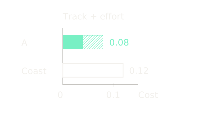
Compare A with coasting, which keeps speed at 0.4 m/s throughout. The bars share a scale of 1,600 drawing units per cost unit. Solid or plain outlined portions represent tracking error; the hatched portion represents effort. Use this deliberately small objective:

$J=\sum_{j=1}^{3}(v_j-0.6)^2+0.005\sum_{k=0}^{2}a_k^2.$

The weight 0.005 has units of seconds squared so both terms have matching units. It is a teaching choice. For A, tracking contributes $0^2+0^2+(-0.2)^2=0.04$, and effort contributes $0.005(2^2+0^2+(-2)^2)=0.04$. Thus $J_A=0.08$. Coasting gives $J_B=3(-0.2)^2+0=0.12$.

A wins this two-candidate comparison; it is not the optimal MPC solution. Its last braking action is unnecessary for maintaining the target in this simplified example. Actual optimization searches the allowed sequences, with dynamics and constraints enforced together. MIT's trajectory optimization chapter gives the broader finite-horizon formulation.

A longer horizon can see a coming support change, but adds optimization work. Weights decide how much tracking error is worth reducing for extra effort. Adding a terminal cost can value the state beyond the final interval; a finite horizon and repeated replanning alone do not prove stability.

Keep force inside available grip

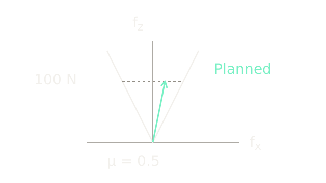
This is force space, not a picture of a leg. The upward axis is normal force $f_z$; the horizontal axis is forward tangential force $f_x$. Both use 1.2 drawing units per newton. The two white boundaries enclose a two-dimensional slice of the friction cone:

$f_z\geq0,\qquad |f_x|\leq\mu f_z.$

The coefficient $\mu$ models available friction. With $\mu=0.5$ and $f_z=100$ N, each foot may supply at most 50 N forward or backward. Our planned 20 N lies inside. The dashed 100 N slice spans the allowed range; the mint vector ends at $(20,100)$ N. The ground can push upward, but this nonadhesive contact cannot pull downward.

In three dimensions, tangential magnitude is $\sqrt{f_x^2+f_y^2}$. A quadratic-program controller can use a conservative inner polyhedral approximation of the circular cone. Independently allowing both tangential components up to $\mu f_z$ instead admits corner forces outside it. Friction, unilaterality and contact models are developed in the legged robotics modeling chapter.

With a fixed schedule, a linearized or prescribed linear prediction model, a convex quadratic cost and linear force constraints, this restricted problem can be a convex quadratic program. Optimizing contact choices or general nonlinear body rotations does not inherit that guarantee.

Redistribute load to turn

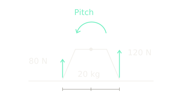
Switch to a separate planar snapshot with purely vertical contact forces. The dot is the center of mass. Rear and front contacts are 0.25 m behind and ahead, drawn at 400 units per metre. The rear supports 80 N and the front 120 N; arrow lengths use 0.8 drawing units per newton.

Their sum remains 200 N, but their turning effects differ. Taking counterclockwise as positive in the drawn horizontal–vertical plane:

$M=0.25(120)-0.25(80)=10\text{ N m}.$

The curved arrow indicates this moment's direction, not a predicted rotation angle. In three dimensions, each contact contributes $\mathbf r_i\times\mathbf f_i$ to the rate of angular momentum; $\mathbf r_i$ runs from center of mass to contact, and $\mathbf f_i$ is that contact's force. Holding position and controlling attitude therefore require more than matching total upward force. The pure-vertical assumption here deliberately removes the pitch moments that horizontal forces would also create.

Execute once, then measure again

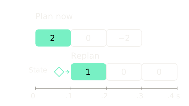
Each cell spans 0.1 seconds. Numbers are accelerations in m/s²; a filled cell marks the first action to execute. Outlined cells remain predictions. After the first interval, the window advances and gets a new final interval. The diamond supplies an updated state estimate.

Suppose the measured speed is 0.5 m/s instead of the predicted 0.6. From that new state, the illustrated replacement candidate $[1,0,0]$ reaches $0.5+1(0.1)=0.6$ m/s, then holds it. That candidate is again an illustration, not a computed optimum. Executing the original remaining $[0,-2]$ would instead leave speed at 0.5 and then reduce it to 0.3 m/s.

This is the feedback in receding horizon control: each solve starts from current estimated state. The unused tail can seed the next solve but is not a commitment. See state estimation for how sensing and prediction combine. An old estimate, missed deadline or infeasible solve still needs an explicit handling policy; repeating optimization does not remove those failures.

Turn forces into motor commands

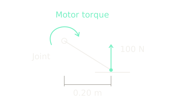
Zoom into an idealized local joint. A 100 N upward foot force acts 0.20 m horizontally from it, so the generalized external joint load is $0.20(100)=20$ N m counterclockwise in the drawn plane. Neglecting gravity and inertia of this local link, the motor must supply 20 N m clockwise to hold it. The arrow shows that opposing motor torque.

For multiple joints, the contact contribution is $\boldsymbol\tau_{ext}=J_c^T\mathbf f$, where $J_c$ maps joint velocity to foot velocity in a consistent coordinate frame. This external load must be combined with the full dynamics; actuator compensation uses the corresponding opposing sign. A force plan alone does not provide swing-foot tracking or verify motor limits.

A whole-body controller can reconcile planned forces with body motion, swing legs and joint commands. Kim and colleagues describe this split in whole-body impulse control with MPC. The trade-off is model detail and computation versus responsiveness: a compact body planner is easier to optimize, while execution still needs joint-level feedback and feasibility checks. PID feedback illustrates that lower-level correction and saturation.

Where it breaks

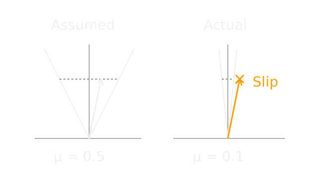
Both panels use identical force scales and request the same $(20,100)$ N. The left assumes $\mu=0.5$, allowing 50 N tangential force. The actual surface on the right has $\mu=0.1$, allowing only 10 N. The requested 20 N lies outside the narrower cone; the cross marks the violated bound. These coefficients are synthetic, not measured material properties.

At the pictured 100 N normal load, each foot can sustain only half the requested forward force without exceeding the assumed static-friction bound. Keeping two such loads gives a 20 N total tangential limit and at most $20/20=1$ m/s² forward acceleration, versus the planned 2. The predicted velocity and contact locations are no longer trustworthy if a foot slides.

Replanning can reduce the demand, change support or seek a new foothold only when those options remain physically feasible. It cannot manufacture grip. Touchdown error, actuator saturation, unmodeled impacts and delay can likewise invalidate a prediction. For an uncomplicated fixed stance with small disturbances, simpler feedback may be sufficient; predictive optimization earns its cost when upcoming constraints and support changes affect today's action.

The Quick Version

• Stance contacts transmit ground forces; swing feet do not.
• Net external force determines center-of-mass acceleration.
• A prescribed gait restricts which feet may exert force.
• A dynamics model predicts candidate motion across a finite horizon.
• Tracking and effort weights rank feasible candidate sequences.
• Friction limits the tangential force each contact can support.
• Force distribution also controls the body's angular momentum.
• MPC executes the first action, then replans from updated state.
• Joint control must realize planned forces within actuator limits.
• Wrong contact assumptions can make optimized predictions physically infeasible.