Compressive Sensing

Why Does This Exist?

Sample-then-discard is everywhere: cameras grab megapixels JPEG shrinks hundredfold, MRI fills k-space for hours to keep a fraction. Where sampling is slow, expensive, or irradiating (MRI scan time, terahertz cost, single-photon budgets), oversampling first and compressing later wastes the scarcest resource.

Compressive sensing measures compressively from the start: $m$ random projections with $m$ far below the pixel count $n$, then reconstructs by seeking the sparsest signal consistent with the measurements. MRI acceleration, single-pixel cameras, and lensless imagers run on it. The software-camera sibling is computational photography; the map is alternative sensing.

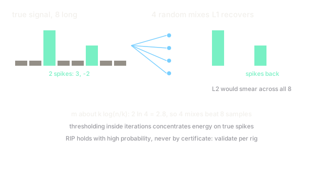
The one idea you need first. A signal is $k$-sparse if only $k$ of its $n$ coefficients are nonzero in some basis (wavelets for photos). L1 minimization finds the measurement-consistent signal with the smallest absolute sum — and that sum lightly penalizes spread-out energy while tolerating concentrated spikes, so the optimum lands on few nonzeros. L2 instead spreads energy everywhere; the norm choice is the algorithm.

Think of It Like This

How It Actually Works

Model $y = \Phi x$ with $\Phi$ an $m \times n$ random matrix ($m \ll n$). Assume $x = \Psi s$ with $s$ $k$-sparse. Solve $\min \lVert s\rVert_1$ subject to $y = \Phi\Psi s$ via iterative thresholding or linear programming. Theory (restricted isometry: $\Phi\Psi$ nearly preserves lengths of sparse vectors) says $m \sim k\log(n/k)$ measurements suffice — far below Nyquist's $n$. Practice designs $\Phi$ in hardware (coded apertures, micromirror patterns, k-space trajectories) and $\Psi$ from the domain (wavelets, gradients, learned dictionaries).

Recovery is iterative and slow next to a shutter click; that compute bill is the standing tradeoff.

Worked example

Signal length $n = 8$ with $k = 2$ nonzeros (values $3$ at position $2$, $-2$ at position $5$). Measurement budget $m \approx k\log(n/k) = 2\ln(4) \approx 2 \times 1.39 = 2.77$, so $3$–$4$ projections should suffice — half the Nyquist $8$.

Soft thresholding shows the sparsity mechanism on a noisy coefficient vector $[0.8, -0.1, 0.05]$ at threshold $0.2$: survivors keep magnitude-minus-threshold with sign ($0.8 \to 0.6$), and anything below dies ($-0.1 \to 0$, $0.05 \to 0$). Repeated inside iterations, this operator is what concentrates energy onto the true spikes while L2 would shrink everything proportionally and smear on.

Code

The point of this snippet is the concentration operator: thresholding kills small fry and keeps spikes standing.

1def soft_threshold(values: list, lam: float) -> list:2    out = []3    for v in values:  # shrink toward zero, kill below lambda4        kept = abs(v) - lam5        out.append(0.0 if kept <= 0 else (1.0 if v > 0 else -1.0) * kept)6    return out7
8
9print(soft_threshold([0.8, -0.1, 0.05], 0.2))  # -> [0.6, 0.0, 0.0]

Watch Out For

The Quick Version

• Compressive sensing measures $m \ll n$ random projections and reconstructs via sparsity-seeking L1.
• The worked fixture budgets $3$–$4$ measurements for $2$ spikes in length $8$, versus $8$ Nyquist samples.
• Soft thresholding concentrates energy on true spikes where L2 would smear it everywhere.
• RIP guarantees are probabilistic for real matrices, so validate per setup with known targets.
• Quote measure-plus-solve latency: iterative reconstruction lags far behind sensor rates.

What to Read Next

• Computational Photography
• Event and Alternative Sensing