DeepLab v1 to v3 Plus

DeepLab keeps resolution high with atrous convolutions, sees many scales at once with ASPP, and sharpens edges with a small decoder in v3 Plus.

DeepLab holds the feature map at high resolution with spaced-out filters and probes it with parallel pooling branches at several scales.

Why Does This Exist?

Downsampling by $32$ throws away the exact pixels semantic segmentation must label, and one fixed filter scale misses objects that range from a distant pedestrian to a near bus. The DeepLab line (Chen et al., 2015 to 2018) attacked both without exploding compute: hold the output stride at $8$ or $16$ with spaced-out filters, then probe every location at several fields of view at once.

This page traces v1 through v3 Plus as one arc. For the competing pyramid-pooling answer see PSPNet, and for object-context refinement see OCRNet.

Think of It Like This

A surveyor with a zoom rake

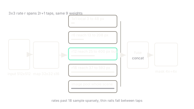
A surveyor must map pebbles and boulders in one pass. A normal rake touches adjacent soil only. An atrous rake skips teeth: same handle weight, wider reach. ASPP hands the surveyor four rakes at once with gaps of $6$ , $12$ and $18$ inches plus a whole-field glance, then merges the readings. v3 Plus adds a fine brush for the pebble outlines.

Where it stops: wider gaps sample sparsely, so very thin structures can fall between the teeth.

How It Actually Works

Atrous convolution

A $3 \times 3$ filter with dilation rate $r$ inserts $r - 1$ gaps between taps, reaching $(2r + 1)$ pixels across with $9$ weights. Rate $2$ covers $5 \times 5$ ; rate $6$ covers $13 \times 13$ . DeepLab replaces striding in the last blocks with dilation, so output stride stays $16$ (v1/v2) or $8$ (v3) instead of $32$ .

ASPP and the version ladder

v1 pairs atrous convolutions with a dense CRF that snaps labels to image edges. v2 introduces Atrous Spatial Pyramid Pooling: parallel $3 \times 3$ branches at rates $6$ , $12$ , $18$ , $24$ plus a $1 \times 1$ branch, concatenated and fused. v3 drops the CRF, adds image-level pooling, and batches normalization. v3 Plus adds a light decoder that upsamples the ASPP output $4\times$ and fuses it with low-level backbone features before the final $4\times$ stretch.

Worked example

Backbone at output stride $16$ on a $512 \times 512$ image gives a $32 \times 32$ map. An ASPP branch at rate $12$ has field $25 \times 25$ on that map, which is $25 \times 16 = 400$ input pixels across: enough to cover a bus. The rate- $6$ branch covers $13 \times 16 = 208$ pixels for cars. The $1 \times 1$ branch reads local texture. Concatenated, one location votes bus, car, and road texture together, and the v3 Plus decoder re-snaps the winning vote to the low-level edge map.

Code

1# Atrous reach: a 3x3 kernel with rate r covers (2r+1) map pixels.2def reach(rate: int) -> int:3    return 2 * rate + 14
5rates = [1, 6, 12, 18]6print([(r, reach(r), reach(r) * 16) for r in rates])7# -> [(1, 3, 48), (6, 13, 208), (12, 25, 400), (18, 37, 592)]

Watch Out For

Gridding artefacts at large rates

Rates above $18$ on a stride- $16$ map sample isolated pixels with dead gaps between taps. Symptom: striped misses on thin rails and wires. Fix: cap rates near the map size, add the image-pooling branch, or switch output stride to $8$ .

Shipping v1 CRF settings with v3

The dense CRF helped v1 but v3 Plus is accurate without it, and stale CRF sigmas blur the new sharp edges. Symptom: worse boundaries after adding post-processing. Fix: retune or drop the CRF when moving to v3 or v3 Plus.

The Quick Version

Atrous convolution widens the receptive field with no extra weights and no extra downsampling.
ASPP probes each location at rates $6$ , $12$ , $18$ plus image pooling to catch many object scales.
v1 used a dense CRF; v2 added ASPP; v3 modernized training; v3 Plus added a light edge decoder.
Output stride $8$ or $16$ keeps maps dense enough for boundaries.
Over-large dilation rates cause gridding on thin structures.