Fully Convolutional Networks

Fully convolutional networks turned a classifier into a dense pixel labeller by swapping fully connected layers for 1x1 convolutions plus learned upsampling.

FCN converts class scores into a coarse grid and learns to upsample it back to a full-resolution pixel mask.

Why Does This Exist?

Image classifiers output one label per image, but semantic segmentation needs one label per pixel. The obvious fix of running a classifier on every sliding window repeats work thousands of times and still outputs blocky maps.

FCN (Long, Shelhamer, Darrell, 2015) showed the classifier already computes a spatial grid before its final layers. Convert those layers to convolutions, add learned upsampling, and the whole image is labelled in one forward pass. This page covers the conversion trick and the FCN-32s/16s/8s ladder. Neighbours cover the successors: SegNet for pooling indices and DeepLab for atrous context.

Think of It Like This

A rubber stamp grid instead of one stamp at a time

Imagine grading a wall of exam papers pinned in a grid. The old way picks up one paper, stamps it, puts it back, and repeats 10,000 times. FCN is a stamp as wide as the wall: one press grades every paper at once, then a second expanding press sharpens the blurry edges back to full size.

Where it stops: the giant stamp still sees coarsely, so fine edges need the skip fusions described below.

How It Actually Works

A VGG-style backbone downsamples a $H \times W$ image by $32$ through five pooling stages, ending with a $H/32 \times W/32 \times 4096$ tensor. A fully connected layer reads that whole tensor at once, which is why it destroys spatial layout.

The convolutionalization trick

Replace each fully connected layer with a $1 \times 1$ convolution with the same weights. A layer that mapped $4096$ inputs to $1000$ scores becomes $1000$ filters of size $1 \times 1$ . The output changes from a $1000$ -vector to a $H/32 \times W/32 \times K$ score grid with $K$ classes. Nothing is relearned; the weights are reshaped, so ImageNet pretraining carries over.

Learned upsampling and the 32s/16s/8s ladder

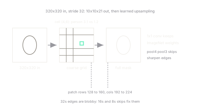
A transposed convolution with stride $32$ stretches the coarse grid back to $H \times W$ (FCN-32s), but edges are blobby. FCN-16s upsamples $2\times$ , adds the pool4 prediction map, then upsamples $16\times$ . FCN-8s repeats from pool3. Each skip re-injects a sharper map before the final stretch.

Worked example

Input $320 \times 320$ . Backbone output is $10 \times 10 \times 21$ for $21$ PASCAL classes. A pixel at coarse position $(4, 6)$ with winning class $15$ (person) and score $3.1$ vs runner-up $1.2$ covers a $32 \times 32$ patch in the input, rows $128$ to $159$ , columns $192$ to $223$ . Bilinear initialization of the transposed filter spreads that $3.1$ smoothly, and the pool3 skip (at $40 \times 40$ ) corrects the patch border by up to $4$ pixels where the person meets the background.

Code

1# Coarse-grid geometry of FCN-32s on a 320x320 input.2H, W, stride, classes = 320, 320, 32, 213gh, gw = H // stride, W // stride4print((gh, gw, classes))5# -> (10, 10, 21)6
7# Input patch covered by coarse cell (4, 6).8r, c = 4, 69print((r * stride, (r + 1) * stride, c * stride, (c + 1) * stride))10# -> (128, 160, 192, 224)

Watch Out For

Checkerboard artefacts from transposed convolutions

Stride- $32$ transposed convolutions with uneven kernel overlap paint a faint grid over the mask. Symptom: regular checkerboard flicker on flat regions like sky. Fix: initialize with bilinear weights, keep kernel size divisible by stride, or upsample with bilinear interpolation followed by a $1 \times 1$ convolution.

Treating FCN-32s output as boundary truth

Coarse-only FCN-32s is off by many pixels at edges. Do not measure thin structures with it. Move to FCN-8s skips or a later encoder-decoder design before trusting boundaries.

The Quick Version

FCN replaces fully connected layers with $1 \times 1$ convolutions, keeping ImageNet weights and producing a spatial score grid.
Transposed convolutions learn the upsampling from $1/32$ resolution back to full size.
FCN-16s and FCN-8s fuse pool4 and pool3 maps to sharpen boundaries.
One forward pass labels the whole image instead of thousands of sliding windows.
Coarse-only output is blobby; skips or later decoders fix the edges.