Denoising Autoencoder

A denoising autoencoder learns by cleaning up deliberately corrupted images, so its bottleneck keeps only the structure that survives the damage.

Why Does This Exist?

A plain autoencoder can cheat. If its bottleneck is wide enough, it memorises the input pixel for pixel and learns nothing useful about structure. The reconstructions look perfect and the features are worthless.

Corruption removes the cheat. When salt-and-pepper noise blanks out a fifth of every training image, memorisation no longer works: the network cannot copy pixels it never saw. To rebuild the clean original it must learn what images in this dataset typically look like, which strokes continue, which textures repeat. That pressure is the whole point, and it is why denoising autoencoders became a pretraining workhorse before large labelled datasets were common.

This page teaches that one training trick. The plain autoencoder it builds on lives in autoencoders, and the sibling sparse autoencoder constrains the bottleneck a different way.

Think of It Like This

Restoring a photo with coffee stains

You get a family photo with coffee splattered across it. You cannot see every face, but you know how faces work: two eyes, symmetry, skin tones that continue under the stain. You fill in each blotch with what must have been there.

A friend who only ever saw pristine photos could copy them exactly but would freeze at the first stain. You learned the actual structure of faces because damage forced you to. The corruption is the teacher, not the obstacle, and it stops helping the day the network can undo it without understanding, which is where the limits below come in.

How It Actually Works

Write the clean input $x$ (an image flattened to a vector). Sample a corruption process $C$ , for example masking noise that zeroes each pixel independently with probability $p = 0.2$ , and train on the corrupted copy $\tilde{x} = C(x)$ . The network has an encoder $f$ and a decoder $g$ :

\hat{x} = g(f(\tilde{x})), \qquad L = \lVert \hat{x} - x \rVert^2

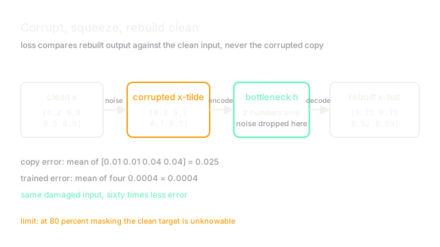
Three symbols: $x$ is the clean target the loss compares against, $\tilde{x}$ is the damaged input the encoder actually sees, and $\hat{x}$ is the reconstruction. The loss always measures against the clean $x$ , never against the corrupted copy. Training on $\tilde{x} \to \tilde{x}$ would teach the network to reproduce damage.

Why the bottleneck learns structure

The encoder output $h = f(\tilde{x})$ is narrow, far fewer numbers than the input pixels. Information the network wants to keep about $x$ must survive that squeeze. Pixel-level noise is nearly incompressible, it looks different every batch, so the squeeze discards it first. Stable structure, edges, shapes, palettes, survives because the decoder can regenerate whole regions from a compact description of them.

Worked example

Take a four-pixel signal $x = [0.2, 0.8, 0.5, 0.9]$ and masking noise $n = [0.1, -0.1, 0.2, -0.2]$ , giving $\tilde{x} = [0.3, 0.7, 0.7, 0.7]$ . Before training, copying the input gives mean squared error $\text{mean}([0.01, 0.01, 0.04, 0.04]) = 0.025$ .

A trained denoising autoencoder outputs $\hat{x} = [0.22, 0.78, 0.52, 0.88]$ . Each error is $0.02$ , each square is $0.0004$ , so the mean is $0.0004$ . Same corrupted input, sixty times less error, because the bottleneck kept the signal pattern and dropped the noise pattern.

Code

The corruption step is three lines. Everything else is a standard autoencoder, which is exactly the point: the trick is in the data, not the architecture.

1import random2
3
4def corrupt(x: list[float], p: float = 0.25, seed: int = 1) -> list[float]:5    """Zero each entry independently with probability p (masking noise)."""6    rng = random.Random(seed)7    return [0.0 if rng.random() < p else v for v in x]8
9
10x = [0.2, 0.8, 0.5, 0.9]11print(corrupt(x))  # -> [0.0, 0.8, 0.5, 0.9]

Watch Out For

Corruption so heavy the target becomes unknowable

Push the masking rate to $p = 0.8$ and reconstructions turn to mush, not because the network is weak but because the task is impossible: with four of five pixels gone, several plausible clean images fit the same corrupted input. The loss stays high forever and people blame the architecture.

Start near $p = 0.2$ for masking noise or small Gaussian $\sigma$ , and raise it only while validation reconstruction keeps improving. The corruption should hide detail, never delete the subject.

Evaluating on corrupted inputs by accident

The validation pipeline must corrupt inputs but score against clean targets, exactly like training. Score $\hat{x}$ against $\tilde{x}$ and a model that faithfully reproduces noise looks better than one that removes it, which inverts the entire ranking.

Keep clean targets alongside every validation batch and assert the scorer reads those, not the corrupted copies.

The Quick Version

A denoising autoencoder trains on corrupted input but scores against the clean original, so copying is not an option.
The narrow bottleneck keeps compressible structure and drops incompressible noise first.
Masking noise near $p = 0.2$ or small Gaussian noise is the usual starting corruption.
Our toy signal drops from $0.025$ copy error to $0.0004$ reconstruction error after training.
Too much corruption makes the target unknowable, and validation must score against clean images.