EfficientNet Compound Scaling

EfficientNet scales depth, width and resolution together with one knob, so each bigger model spends its extra budget where it helps instead of on depth alone.

Scaling depth, width and resolution together with 1.2, 1.1 and 1.15 doubles FLOPs per step and lifts B0 to 77 percent top 1 with 5.3M weights.

Why Does This Exist?

Scaling one dimension stalls. Deeper-only ResNets gain little past 200 layers, wider-only nets memorize, and higher resolution alone feeds detail the network has no capacity to use. Teams scaled whatever was easiest and paid full price for shrinking gains.

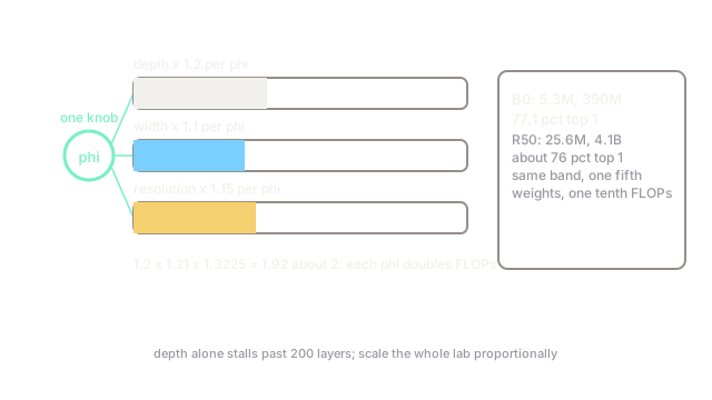
EfficientNet (Tan and Le, 2019) scales all three together with compound coefficient $\phi$ : depth by $\alpha^{\phi}$ , width by $\beta^{\phi}$ , resolution by $\gamma^{\phi}$ with $\alpha \cdot \beta^2 \cdot \gamma^2 \approx 2$ so each step doubles FLOPs. The B0 baseline uses mobile inverted bottleneck blocks with squeeze-excitation, and B1 through B7 walk $\phi$ upward. This page covers the scaling rule. Phone-grade blocks live in MobileNet and the residual backbone in residual networks.

Think of It Like This

Enlarging a photo lab, not one machine

A photo lab doubling output cannot just buy developers. It needs proportionally more enlargers (depth), wider paper stock (width) and finer-grained film (resolution). One without the others jams the line.

Compound scaling is the proportional order. Depth-only scaling is buying developers while the enlargers queue up untouched.

How It Actually Works

The found coefficients are $\alpha = 1.2$ , $\beta = 1.1$ , $\gamma = 1.15$ . Check the constraint: $1.2 \times 1.1^2 \times 1.15^2 = 1.2 \times 1.21 \times 1.3225 \approx 1.92$ , near 2, so $\phi = 1$ doubles FLOPs. B0 at 224 resolution grows to B4 at 380 with $\phi = 4$ , roughly $2^4 = 16$ times the FLOPs for a large accuracy step instead of the 16x-depth alternative that stalls.

B0 itself is concrete: about 5.3 million parameters and 390 million FLOPs at roughly 77.1% top-1 on ImageNet, against ResNet-50 at 25.6 million parameters and 4.1 billion FLOPs near 76%. Same accuracy band at one fifth the weights and one tenth the compute. V2 later replaced early MBConv blocks with fused convolutions because depthwise steps on large early maps pay high memory-access cost for little arithmetic.

Code

1alpha, beta, gamma = 1.2, 1.1, 1.152print(round(alpha * beta**2 * gamma**2, 2))3# -> 1.924
5b0_flops = 390_000_0006print(b0_flops * (2 ** 4) // 1_000_000)7# -> 6240

Watch Out For

Scaling resolution past what the objects support

Raising input to 600 on 32x32-object data adds FLOPs with no new signal. The symptom is slower training and flat accuracy. Hold resolution fixed when objects are small and spend the budget on width instead.

Copying B7 training settings onto B0 fine-tuning

Large EfficientNets need RMSProp with strong AutoAugment and stochastic depth; small ones fine-tune best with lighter augmentation and shorter schedules. The symptom is a B0 that underfits under B7 regularization. Match the schedule to the model size being trained.

The Quick Version

EfficientNet scales depth, width and resolution together so each doubling of FLOPs buys real accuracy.
Coefficients 1.2, 1.1 and 1.15 satisfy the doubling constraint at about 1.92 per step.
B0 matches ResNet-50 accuracy near 77% with 5.3 million parameters against 25.6 million.
MBConv blocks with squeeze-excitation carry the efficiency; V2 fuses early blocks for memory access.
Scale resolution only when objects are large enough to reward it.