Residual and Dense Networks

Instead of learning a full mapping from scratch, skip connections let layers learn only the residual difference, enabling networks hundreds of layers deep.

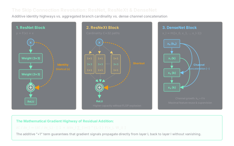
Architectural blueprints of ResNet identity skip connections, ResNeXt multi-branch cardinality, and DenseNet dense feature concatenation.

Why Does This Exist?

When deep neural networks were pushed past 20 layers in the mid-2010s, researchers observed a counterintuitive failure mode: the degradation problem. As network depth increased, training accuracy did not merely saturate—it dramatically worsened. A 56-layer plain convolutional network suffered higher training error and higher test error than a shallower 20-layer counterpart on CIFAR-10.

This failure was not caused by overfitting (since training error itself was higher) nor solely by vanishing gradients (which normalized initializations and Batch Normalization had largely stabilized). Instead, deep plain networks were mathematically incapable of learning simple identity mappings. If the optimal depth for a visual task is 20 layers, adding 36 additional layers should theoretically leave performance unchanged if those extra layers simply pass inputs through unmodified ( $H(x) = x$ ). In practice, fitting an identity mapping using non-linear weight layers $W_2 \sigma(W_1 x)$ is extremely difficult for gradient descent to discover.

Residual Networks (ResNet, He et al., 2015) revolutionized deep learning by introducing identity shortcut connections. Instead of forcing layers to fit an underlying mapping $\mathcal{H}(x)$ , the network explicitly fits a residual function $\mathcal{F}(x) = \mathcal{H}(x) - x$ , outputting $\mathcal{H}(x) = \mathcal{F}(x) + x$ . This simple additive skip connection enabled networks to scale stably to 152 layers, and eventually over 1,000 layers. Subsequent architectures like ResNeXt (Xie et al., 2017) and DenseNet (Huang et al., 2017) extended this principle through multi-branch cardinality and dense feature-concatenation highways.

Think of It Like This

A manuscript editing pipeline with original carbon copies

Imagine writing a 150-page legal manuscript through a team of 150 sequential junior editors. In a plain network, each editor retypes the entire manuscript from memory based on the previous editor's draft. By editor 30, small omissions, phrasing shifts, and typos compound into garbled noise. If an editor has nothing useful to add, they struggle to produce an exact word-for-word copy of what they read.

A residual network clips the original draft to every editor's desk. Each editor is instructed only to mark red-pen corrections (the residual $\mathcal{F}(x)$ ) on an overlay sheet. If an editor has no improvements to make, they leave the overlay completely blank ( $\mathcal{F}(x) = 0$ ), and the original document passes forward cleanly intact.

DenseNet takes this even further: instead of just receiving the draft from the immediately preceding editor, every single editor receives a complete folder containing the drafts written by every prior editor in the chain, allowing anyone to reference early raw sketches alongside recent revisions.

How It Actually Works

The ResNet Formulation and Gradient Highway

Formally, a residual building block computes:

y = \mathcal{F}(x, \{W_i\}) + x

where $x$ and $y$ are the input and output vectors, and $\mathcal{F}$ is the residual mapping to be learned. When input and output channel dimensions differ (or when downsampling via stride), a linear projection $W_s$ aligns the shortcut:

y = \mathcal{F}(x, \{W_i\}) + W_s x

For an arbitrary deep layer $L$ relative to an earlier layer $l$ , the forward state is:

x_L = x_l + \sum_{i=l}^{L-1} \mathcal{F}(x_i, \mathcal{W}_i)

During backpropagation, let $\mathcal{E}$ denote the scalar loss function. Applying the multivariable chain rule yields:

\frac{\partial \mathcal{E}}{\partial x_l} = \frac{\partial \mathcal{E}}{\partial x_L} \frac{\partial x_L}{\partial x_l} = \frac{\partial \mathcal{E}}{\partial x_L} \left( \mathbf{I} + \frac{\partial}{\partial x_l} \sum_{i=l}^{L-1} \mathcal{F}(x_i, \mathcal{W}_i) \right)

The identity matrix $\mathbf{I}$ creates an uninterrupted gradient highway. Even if the weight gradient term $\frac{\partial}{\partial x_l} \sum \mathcal{F}$ diminishes to zero, the gradient $\frac{\partial \mathcal{E}}{\partial x_L}$ propagates directly back to layer $l$ without vanishing.

ResNeXt: Aggregated Residual Transformations and Cardinality

ResNeXt replaces the two-layer or three-layer bottleneck in ResNet with a set of $C$ parallel homogeneous transformations (termed cardinality):

y = x + \sum_{i=1}^{C} \mathcal{T}_i(x)

Each path $\mathcal{T}_i(x)$ performs a low-dimensional bottleneck projection ( $1 \times 1 \to 3 \times 3 \to 1 \times 1$ ). Rather than simply increasing network depth or channel width, increasing cardinality $C$ (typically $C=32$ ) increases representational capacity much more effectively without expanding FLOP count or parameter complexity. ResNeXt is mathematically equivalent to grouped convolutions with group count equal to $C$ .

DenseNet: Connecting Every Layer to Every Other Layer

DenseNet shifts from additive shortcuts ( $+$ ) to channel concatenation ( $[\cdot]$ ). For a block with $L$ layers, each layer receives the feature maps of all preceding layers as input:

x_l = H_l\left(\left[ x_0, x_1, x_2, \ldots, x_{l-1} \right]\right)

If each function $H_l$ produces $k$ feature maps, the input to layer $l$ has $k_0 + k \times (l - 1)$ channels, where $k$ is the network growth rate (typically small, e.g., $k = 32$ ). Between dense blocks, transition layers apply a $1 \times 1$ convolution and $2 \times 2$ average pooling with a compression factor $\theta \in (0, 1]$ to control memory footprint.

Worked Example

Let us trace a ResNet bottleneck block taking an input tensor $X \in \mathbb{R}^{256 \times 56 \times 56}$ with stride $S=1$ :

Input shape: $(256, 56, 56)$
Layer 1 (Reduce): Conv2d(256, 64, kernel=1, bias=False) $\to$ $\to$ BatchNorm2d $\to$ $\to$ ReLU
- Output shape: $(64, 56, 56)$
- Parameters: $256 \times 64 \times 1 \times 1 = 16\text{,}384$
Layer 2 (Spatial): Conv2d(64, 64, kernel=3, padding=1, bias=False) $\to$ $\to$ BatchNorm2d $\to$ $\to$ ReLU
- Output shape: $(64, 56, 56)$
- Parameters: $64 \times 64 \times 3 \times 3 = 36\text{,}864$
Layer 3 (Expand): Conv2d(64, 256, kernel=1, bias=False) $\to$ $\to$ BatchNorm2d
- Output shape: $(256, 56, 56)$
- Parameters: $64 \times 256 \times 1 \times 1 = 16\text{,}384$
Shortcut: Identity connection (since shapes match: $256 = 256$ $256 = 256$ , $S=1$ $S = 1$ )
- Output: $\mathcal{F}(X) + X$
- Final shape after ReLU: $(256, 56, 56)$

Total parameters in this bottleneck: $16\text{,}384 + 36\text{,}864 + 16\text{,}384 = 69\text{,}632$ weights (excluding BatchNorm affine parameters). If we had used two plain $3 \times 3$ convolutions with 256 channels, it would have cost $2 \times (256 \times 256 \times 9) = 1\text{,}179\text{,}648$ parameters—over $16\times$ more parameters!

Code

1import torch2import torch.nn as nn3
4class ResNetBottleneck(nn.Module):5    """Standard ResNet bottleneck block with additive identity shortcut."""6    def __init__(self, in_channels: int, mid_channels: int, stride: int = 1) -> None:7        super().__init__()8        out_channels = mid_channels * 49        10        self.conv1 = nn.Conv2d(in_channels, mid_channels, kernel_size=1, bias=False)11        self.bn1 = nn.BatchNorm2d(mid_channels)12        self.conv2 = nn.Conv2d(mid_channels, mid_channels, kernel_size=3, stride=stride, padding=1, bias=False)13        self.bn2 = nn.BatchNorm2d(mid_channels)14        self.conv3 = nn.Conv2d(mid_channels, out_channels, kernel_size=1, bias=False)15        self.bn3 = nn.BatchNorm2d(out_channels)16        self.relu = nn.ReLU(inplace=True)17        18        # Shortcut projection if spatial dimension or channel count changes19        if stride != 1 or in_channels != out_channels:20            self.shortcut = nn.Sequential(21                nn.Conv2d(in_channels, out_channels, kernel_size=1, stride=stride, bias=False),22                nn.BatchNorm2d(out_channels)23            )24        else:25            self.shortcut = nn.Identity()26
27    def forward(self, x: torch.Tensor) -> torch.Tensor:28        identity = self.shortcut(x)29        30        out = self.relu(self.bn1(self.conv1(x)))31        out = self.relu(self.bn2(self.conv2(out)))32        out = self.bn3(self.conv3(out))33        34        out += identity35        return self.relu(out)36
37# Verification with Batch=2, Channels=256, Height=56, Width=5638x = torch.randn(2, 256, 56, 56)39block = ResNetBottleneck(in_channels=256, mid_channels=64, stride=1)40out = block(x)41
42print(out.shape)43# -> torch.Size([2, 256, 56, 56])

Watch Out For

In-place activation corruption on residual skip tensors

A notorious runtime error occurs when applying PyTorch's in-place nn.ReLU(inplace=True) directly before or during residual accumulation. If the tensor $x$ entering the block is modified in-place by an earlier operation, the identity shortcut $x$ will hold altered activation values by the time out += x executes.

Furthermore, during backpropagation, PyTorch requires the unmodified input $x$ to calculate gradients for the shortcut branch. If $x$ was modified in-place, the backward pass will crash with a RuntimeError: one of the variables needed for gradient computation has been modified by an inplace operation. Never perform in-place mutations on tensors that feed active residual branches.

The Quick Version

ResNet resolves the network degradation problem by reformulating layer objectives to fit residual differences $\mathcal{F}(x) = \mathcal{H}(x) - x$ .
The additive identity shortcut adds an identity matrix term $\mathbf{I}$ to the backpropagation chain rule, preserving clean gradient flow across hundreds of layers.
ResNeXt introduces cardinality (grouped parallel paths) as an architectural dimension that outperforms naive depth and width scaling.
DenseNet replaces addition with channel concatenation, passing every layer's output to all subsequent layers for maximum feature reuse.
Bottleneck designs ( $1 \times 1 \to 3 \times 3 \to 1 \times 1$ ) compress channels before expensive spatial convolutions, dramatically lowering computational cost.