Lucas-Kanade Optical Flow

Lucas-Kanade tracks a point by assuming its whole neighborhood moves together, turning many shaky single-pixel guesses into one steady motion vector.

One window of pixels votes together through least squares, producing a single motion arrow for the tracked corner.

Why Does This Exist?

Optical flow starts from one equation with two unknowns: $I_x u + I_y v + I_t = 0$ , where $I_x, I_y$ are the image gradients, $I_t$ is the change between frames, and $(u, v)$ is the motion you want. One pixel cannot determine its own motion; that is the aperture problem. You need an extra assumption from somewhere.

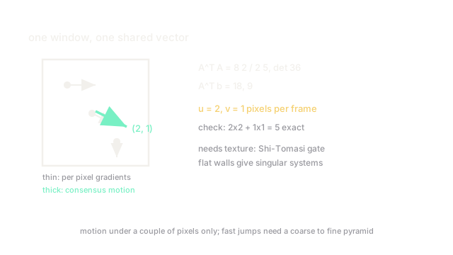
Lucas and Kanade (1981) supplied the most practical one: motion is constant inside a small window. A $5 \times 5$ patch gives 25 equations for the same 2 unknowns, and least squares finds the vector that satisfies them best. Trackers use it on corners and keypoints because textured windows constrain the answer while blank walls do not. It is sparse flow: fast, local, and the backbone of point tracking pipelines.

Think of It Like This

Twenty witnesses, one getaway car

One witness saw a blur and guesses the car went north. Useless alone. But twenty witnesses around the same intersection each caught a fragment, and all fragments agree the car went northeast at speed. You trust the consensus, not any single account.

Each pixel in the window is a witness with one equation. Least squares is the detective combining them: the shared $(u, v)$ that contradicts the fewest accounts wins. And just like witnesses, blank-wall pixels saw nothing and contribute no information, which the math reveals as an unsolvable system.

How It Actually Works

1. Stack the window into a system

For every pixel $k$ in the window, write its constraint $I_{xk} u + I_{yk} v = -I_{tk}$ . Stack them into $A [u, v]^T = b$ with one row per pixel. The least-squares answer is $[u, v]^T = (A^T A)^{-1} A^T b$ , where $A^T A$ is a $2 \times 2$ matrix summarizing the window's texture.

2. Worked example

Three pixels give gradients $(I_x, I_y) = (2, 0), (2, 1), (0, 2)$ with $-I_t$ values $4, 5, 2$ . Then $A^T A = \begin{bmatrix}8 & 2 \\ 2 & 5\end{bmatrix}$ and $A^T b = [18, 9]^T$ . Solving: determinant $36$ , $u = (5 \cdot 18 - 2 \cdot 9)/36 = 2$ , $v = (8 \cdot 9 - 2 \cdot 18)/36 = 1$ . The window moves $(2, 1)$ pixels per frame. Check pixel two: $2 \cdot 2 + 1 \cdot 1 = 5$ . Exact.

3. Good features to track

The solve needs $A^T A$ invertible with large eigenvalues, which happens exactly at corners and textured spots. Shi-Tomasi scoring keeps windows whose smaller eigenvalue clears a threshold and drops edges and flat regions. Pyramids extend the range: solve coarsely at low resolution, refine upward, so large jumps become small ones per level.

Code

1import numpy as np2
3A = np.array([[2, 0], [2, 1], [0, 2]], dtype=float)4b = np.array([4, 5, 2], dtype=float)5u, v = np.linalg.solve(A.T @ A, A.T @ b)6print(u, v)  # -> 2.0 1.0

Watch Out For

Big jumps break the linearization

The constraint equation assumes motion under a couple of pixels; a fast object moves ten and the gradients no longer describe the change. The fix is a coarse-to-fine pyramid, never a bigger window alone. If tracks die on fast motion but survive slow scenes, add pyramid levels.

Flat windows lie confidently

On blank walls $A^T A$ is near-singular and the inverse explodes or returns noise dressed as motion. Always gate on texture (Shi-Tomasi score) before trusting a vector. Horn-Schunck handles blank regions differently, by filling motion in from neighbors.

The Quick Version

Lucas-Kanade assumes one shared motion vector per small window, giving many equations for 2 unknowns.
Least squares solves $(A^T A)^{-1} A^T b$ ; the example window moves $(2, 1)$ pixels.
Only textured windows (corners) constrain the answer; flat regions are unsolvable.
Pyramids extend it to large motions by solving coarse-to-fine.
Sparse and fast: the standard choice for tracking points, not full scenes.