Optical Flow

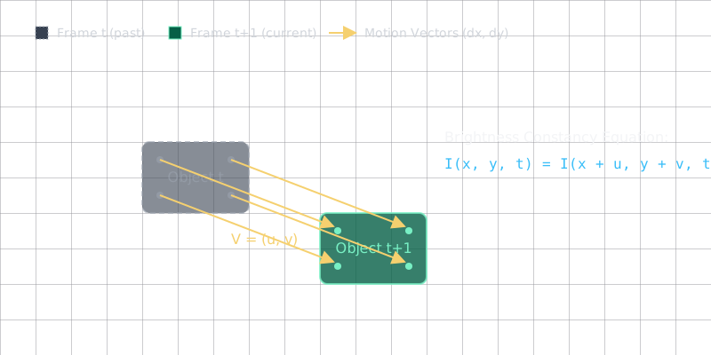
Optical flow estimates where each pixel moved between two video frames, turning a pair of still images into a field of motion arrows.

One pixel shift of (2, 3) satisfies the brightness constraint at all three sample points, which is how a window of pixels pins down both motion components.

Why Does This Exist?

A video is a rapid sequence of still images, and a computer handed two frames has no built-in sense that the car in frame two is the car from frame one. Treating frames as isolated snapshots loses everything action recognition, video compression, navigation and classical object tracking need.

Optical flow bridges the gap by estimating apparent motion per pixel between consecutive frames: the field of arrows that carries each point from where it was to where it went. Sparse methods track a few strong points at frame rate; dense methods fill a vector into every pixel. This page covers the shared constraint equation, the three classical answers and the worked window that shows how two unknowns get pinned down. The sparse sequel is Lucas-Kanade; the modern learned sequel is RAFT.

The one idea you need first. Brightness constancy says a moving point keeps its shade: the pixel that read 145 in frame one still reads 145 in frame two, just somewhere nearby. Every method below is a different way of turning that assumption into motion vectors.

Think of It Like This

Matching footprints across two beach photos

Two aerial photos of a beach show the same crowd minutes apart. Pick one footprint in the first photo, find the identical dent in the second, and draw an arrow between them. Repeat for every dent and the crowd of arrows shows who walked where: long arrows for runners, dots for standers.

Pixels are the dents and brightness is the dent shape you match by. Where it stops: real footprints deform in wet sand and waves erase some entirely, just as lighting changes and occlusions break the constant-brightness bet.

How It Actually Works

The one equation every method shares

Let $I_x$ and $I_y$ be the spatial image gradients (how fast brightness changes moving right and down), $I_t$ the change between frames at that pixel, and $u, v$ the unknown horizontal and vertical displacements. A first-order expansion of brightness constancy gives the optical flow constraint:

$I_x u + I_y v + I_t = 0$

One equation with two unknowns cannot fix a unique $(u, v)$ : that shortfall is the aperture problem, and each method below buys the missing constraint differently.

The three classical answers

Sparse flow (Lucas-Kanade) assumes one shared $(u, v)$ inside each small window and solves the stacked constraints by least squares. It tracks corners and keypoints fast enough for real time and stays silent on blank regions. Global dense flow (Horn-Schunck) demands a smooth field over the whole frame, filling motion into every pixel at the cost of soft boundaries and hundreds of iterations. Local dense flow (Farneback) fits a quadratic brightness surface to each neighborhood and reads the shift from its coefficients, giving dense vectors with no global sweeps.

Worked three-pixel Lucas-Kanade window

Three pixels share motion $(u, v)$ with gradients and temporal changes $(I_x, I_y, I_t)$ equal to $(1, 0, -2)$ , $(0, 1, -3)$ and $(1, 1, -5)$ . Writing $b = -I_t$ per pixel gives $b = [2, 3, 5]$ . Stacking the constraints yields normal equations $A^T A \, [u, v]^T = A^T b$ with:

$A^T A = \begin{bmatrix} 2 & 1 \\ 1 & 2 \end{bmatrix}, \quad A^T b = \begin{bmatrix} 7 \\ 8 \end{bmatrix}$

The determinant is $2 \times 2 - 1 \times 1 = 3$ , so $u = (7 \times 2 - 1 \times 8) / 3 = 6 / 3 = 2$ and $v = (2 \times 8 - 1 \times 7) / 3 = 9 / 3 = 3$ . Checking each pixel: $1 \times 2 + 0 \times 3 - 2 = 0$ , $0 \times 2 + 1 \times 3 - 3 = 0$ , $1 \times 2 + 1 \times 3 - 5 = 0$ . All three residuals vanish, so the window recovers motion $(u, v) = (2, 3)$ exactly: three pixels ganging up is what pins down both components.

Code

1ATA = [[2, 1], [1, 2]]2ATb = [7, 8]3det = ATA[0][0] * ATA[1][1] - ATA[0][1] * ATA[1][0]4u = (ATb[0] * ATA[1][1] - ATA[0][1] * ATb[1]) / det5v = (ATA[0][0] * ATb[1] - ATb[0] * ATA[1][0]) / det6print(det, u, v)7# -> 3 2.0 3.0

Watch Out For

Blank walls defeating the constraint

On smooth, textureless regions the gradients $I_x, I_y$ sit near zero, so the equation constrains almost nothing. The symptom is a flow field that wanders or hallucinates drift across skies and white walls. Fix it by tracking textured corners only, or masking low-gradient regions out of downstream decisions.

Fast motion breaking the small-shift math

The constraint equation is a first-order expansion, valid only for shifts of a pixel or two. The symptom is fast objects that shrink to zero motion or smear across the field. Fix it with coarse-to-fine pyramids that solve big shifts at low resolution first, or learned models such as RAFT for large displacements and occlusions.

The Quick Version

Optical flow estimates per-pixel motion $(u, v)$ between consecutive frames.
Brightness constancy gives one equation, $I_x u + I_y v + I_t = 0$ , for two unknowns.
Lucas-Kanade pools a window by least squares; Horn-Schunck smooths globally; Farneback fits local quadratics.
A three-pixel window with gradients $(1,0)$ , $(0,1)$ , $(1,1)$ recovers motion $(2, 3)$ exactly.
Textureless regions, fast motion and occlusions are the three failure modes to budget for.