Manifold Learning

Face photos of a turning head trace a smooth loop through pixel space, not a cloud. Manifold learning unrolls such curved sheets so distances follow the surface instead of cutting through it.

Graph distance along the curve measures 2.83 while the straight chord claims 2.0, so the embedding respects the surface

Why Does This Exist?

Linear projections fail on curved variation. Photos of one object rotating span a loop in pixel space; PCA flattens the loop into a smear where opposite poses overlap and neighbors in the projection are strangers on the loop. Clustering, retrieval, and visualization built on those distances inherit the error.

Manifold learning assumes the data lies on a low-dimensional curved surface inside the high-dimensional pixel space, and measures distance along the surface (geodesic) instead of through the air (Euclidean). Unrolled correctly, the loop becomes a line where order means pose. The curved-space sibling is hyperbolic embeddings; the shape-invariant sibling is topological data analysis.

The one idea you need first. A k-nearest-neighbor graph connects each image to its few closest neighbors, approximating the surface by short hops. The geodesic distance between two far images is the shortest path through that graph — many small trusted steps instead of one untrusted leap. Isomap embeds points so these graph distances become straight-line distances in few dimensions.

Think of It Like This

An ant on a rolled newspaper

An ant crossing a rolled newspaper walks the curl: around the roll, along the paper, never through the air. A crow flying straight-line distance between the same two points reports a far shorter trip — through space the ant cannot travel.

Euclidean distance is the crow. Geodesic distance is the ant. Manifold learning asks the ant: build the neighbor graph (each step the ant can see), walk it, and lay the walked distances flat. The unrolled newspaper is the embedding, and positions on it mean something walkable, not something flyable.

The analogy stops at the paper's edge: real image manifolds have no neat edges, and choosing how far the ant sees (the neighbor count) decides whether the walk stays on the surface.

How It Actually Works

Isomap runs three steps. First, connect each point to its $k$ nearest neighbors by Euclidean distance, trusting only short hops. Second, compute all-pairs shortest paths through the graph (Dijkstra), giving geodesic estimates. Third, apply classical multidimensional scaling to place points in low dimensions with those path lengths as target distances. Laplacian eigenmaps and LLE vary the third step; the graph-plus-paths idea is shared.

The neighbor count $k$ is the whole game: too small and the graph shatters into islands; too large and long edges tunnel through ambient space, reintroducing the crow's shortcut.

Worked example

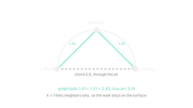
Three photos of a pointer at angles $0$ , $90$ , and $180$ degrees on a unit circle: $A = (1, 0)$ , $B = (0, 1)$ , $C = (-1, 0)$ . The straight chord from $A$ to $C$ measures $2.0$ Euclidean — through the disk, off the manifold. With $k = 1$ , the graph links $A$ – $B$ and $B$ – $C$ (adjacent poses are nearest). Hop lengths: $\lVert A - B\rVert = \sqrt{2} \approx 1.414$ , same for $B$ – $C$ . Shortest path $A \to C$ through $B$ : $1.414 + 1.414 = 2.83$ .

Compare: chord $2.0$ , graph path $2.83$ , true arc $\pi \approx 3.14$ . The graph estimate already respects the curve far better than the chord, and denser sampling closes the remaining gap to the arc.

Code

The point of this snippet is the path estimate: neighbor lists plus one intermediate hop reproduce the $2.83$ geodesic.

1import math2
3
4def dist(p: tuple, q: tuple) -> float:5    return math.hypot(p[0] - q[0], p[1] - q[1])  # straight hop length6
7
8A, B, C = (1.0, 0.0), (0.0, 1.0), (-1.0, 0.0)9chord = dist(A, C)10geodesic = dist(A, B) + dist(B, C)  # shortest path through the graph11print(round(chord, 2))  # -> 2.012print(round(geodesic, 2))  # -> 2.83

Watch Out For

Too few neighbors shatter the surface

With $k$ tiny or data sparse, the graph splits into disconnected islands and shortest paths between islands do not exist. The embedding then places islands arbitrarily, and the arbitrary gaps read as meaningful clusters.

Check connectivity before embedding: one connected component (per true manifold) is the requirement. Raise $k$ or gather denser samples until the graph joins, and distrust any embedding computed over fragments.

Too many neighbors tunnel through the air

With $k$ large, long edges jump across the curve's interior — the crow's shortcut smuggled into the ant's map. Geodesics collapse toward Euclidean chords and the unrolling gains nothing over PCA, while costing far more compute.

Validate $k$ by reconstruction: embed, then check that graph neighbors stay neighbors in the embedding. Sweep $k$ across an order of magnitude; the stable plateau, not any default like $5$ , is the honest setting.

The Quick Version

Manifold learning measures distance along the data surface via neighbor-graph shortest paths.
The worked fixture gives chord $2.0$ , graph path $2.83$ , true arc $3.14$ : the path respects the curve.
Isomap embeds those path lengths in few dimensions; eigenmaps and LLE vary the final step.
Too few neighbors disconnect the graph into meaningless islands; too many tunnel through ambient space.
Sweep the neighbor count and check connectivity before trusting any unrolled map.