Topological Data Analysis in Vision

Counting holes survives stretching, bending, and noisy pixels. Topological data analysis tracks when components merge and loops form as a threshold sweeps, turning shape into a robust signature.

One long persistence bar marks the true loop while short bars mark noise, separating shape from speckle

Why Does This Exist?

Geometric features are brittle. Stretch a digit and template distances explode; add speckle noise and corner counts double; change the threshold and a contour splits in two. Yet a human sees the same "8" through all of it, because the eye counts something stretch-proof: two holes.

Topological data analysis (TDA) counts exactly such invariants. Sweeping a threshold over an image, it records when connected components appear and merge and when loops form and fill. Features that persist across a wide threshold range mark true shape; flickering ones mark noise. The curved-surface sibling is manifold learning; the classical boundary tool is contour detection.

The one idea you need first. Betti numbers count holes by dimension: $\beta_0$ counts connected components, $\beta_1$ counts loops, $\beta_2$ counts enclosed voids. A disk has $\beta_0 = 1, \beta_1 = 0$ . A figure-8 (two loops sharing a point) has $\beta_0 = 1, \beta_1 = 2$ . Persistence tracks each feature's birth threshold $b$ and death threshold $d$ ; the lifetime $d - b$ separates signal from noise.

Think of It Like This

Islands in a rising flood

Watch a mountain range flood in slow motion. At first every peak is its own island ( $\beta_0$ large). Water rises, saddles drown, islands merge. Lakes form inside crater rims ( $\beta_1$ appears), then fill and vanish. Each island and lake has a water level where it is born and one where it dies.

Long-lived islands are the true mountains; ones that flash in and out between two close levels are pebbles. TDA is that flood watch applied to pixel brightness: the threshold is the water level, and persistence (death minus birth) tells mountains from pebbles without ever measuring a single slope.

The analogy stops at the terrain: images have no gravity, and the "water" is an arbitrary intensity sweep whose direction (bright-to-dark or reverse) must be chosen and reported.

How It Actually Works

Build a filtration: threshold the image at increasing levels, adding pixels as they pass. Maintain components with union-find as pixels join (births and merges) and track loops as they enclose and fill. Each feature becomes one interval $[b, d)$ plotted as a bar in the persistence barcode or a point $(b, d)$ in the persistence diagram. Long bars survive to the classifier; short bars near the diagonal are discarded as noise.

Barcodes feed models as vectorized summaries (persistence images, landscapes) or kernel comparisons. The pipeline is deterministic given the filtration, which makes TDA features unusually reproducible next to learned ones.

Worked example

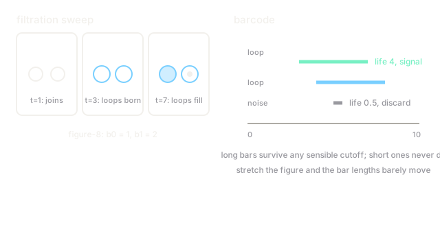
Sweep brightness on a noisy figure-8 image with thresholds $0$ to $10$ :

At $t = 1$ the whole figure connects: one component born, $\beta_0 = 1$ .
At $t = 3$ the left loop encloses: first loop born. At $t = 4$ the right loop encloses: second loop born. Now $\beta_1 = 2$ .
At $t = 7$ both loops fill with brightness: both die. Lifetimes: $7 - 3 = 4$ and $7 - 4 = 3$ .
Speckle noise makes a tiny loop born at $t = 5$ , dead at $t = 5.5$ : lifetime $0.5$ .

Signal lifetimes ( $4$ , $3$ ) tower over the noise ( $0.5$ ). Threshold anywhere sensible and the figure still reads $\beta_1 = 2$ : the count survives the exact threshold choice, which is the robustness classical features lack.

Code

The point of this snippet is the $\beta_0$ count: union-find over a tiny binary grid shows components merging deterministically.

1def count_components(grid: list) -> int:2    parent = {}3
4    def find(a: tuple) -> tuple:5        while parent[a] != a:  # path halving keeps lookups short6            parent[a] = parent[parent[a]]7            a = parent[a]8        return a9
10    for y, row in enumerate(grid):11        for x, v in enumerate(row):12            if v:13                parent[(x, y)] = (x, y)14                for nb in ((x - 1, y), (x, y - 1)):15                    if nb in parent:  # merge with lit neighbors16                        parent[find((x, y))] = find(nb)17    return len({find(p) for p in parent})18
19
20print(count_components([[1, 0, 1], [1, 1, 0], [0, 0, 1]]))  # -> 3

Three lit groups stay three components however the grid stretches: the count is deformation-proof by construction.

Watch Out For

Persistence still needs a scale decision

"Long-lived" is relative: a lifetime of $4$ means nothing without the threshold range ( $0$ – $10$ here) and the noise floor. Teams that threshold barcodes with a magic constant keep different features per dataset and wonder why results do not transfer.

Calibrate on noise: measure lifetimes on shuffled or pure-noise images and keep features clearly above that band. Report the cutoff rule with the result, or the signature is not reproducible.

Full filtrations cost more than the classifier

Naive persistence on megapixel images with fine threshold steps is heavy — easily slower than the downstream model it feeds. Running TDA at full resolution "for accuracy" routinely blows the feature budget.

Downsample first (topology survives), coarsen threshold steps, and restrict to regions of interest. The invariants are coarse by nature; computing them finely wastes the exact robustness you chose TDA for.

The Quick Version

TDA sweeps a threshold and records births and deaths of components ( $\beta_0$ ) and loops ( $\beta_1$ ).
The worked fixture gives loop lifetimes $4$ and $3$ versus noise at $0.5$ : signal separates cleanly.
Long bars mark true shape; short bars near the diagonal mark noise to discard.
Calibrate the lifetime cutoff against noise images instead of using a magic constant.
Downsample before filtering: topology is coarse, so fine computation wastes the budget.