Object Detection

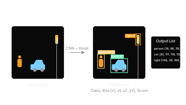
Object detection finds every instance of every object class in an image, returning a bounding box and class label for each — combining classification and localization in a single forward pass.

Why Does This Exist?

Image classification tells you what is in an image. Object detection tells you what is in it and where each instance is located. This is the difference between "there is a person in this image" (classification) and "there are 3 people at these pixel coordinates" (detection).

Autonomous driving, security surveillance, medical imaging, and robotics all need the WHERE, not just the WHAT — and they need it for every object instance simultaneously.

Think of It Like This

A security guard checking every person at a door

A guard checking IDs doesn't just ask "is anyone here authorized?" — they walk up to each person, check their credentials individually, and note their position. Object detection does the same: it scans the image, finds each object instance, classifies it, and records its bounding box coordinates. No object is missed because the scene is complex.

How It Actually Works

Two-stage detection: Faster R-CNN

Faster R-CNN (2015) splits detection into two steps:

Stage 1 — Region Proposal Network (RPN): A small CNN slides over the shared feature map and predicts ~300 region proposals — rectangular regions likely to contain objects. Each proposal has an objectness score and a rough bounding box.

Stage 2 — RoI classification head: RoI pooling extracts a fixed-size feature crop for each proposal from the backbone feature map. A classification head predicts the class label; a regression head refines the bounding box coordinates.

Two-stage detectors are highly accurate but slower (~5–10 FPS on a V100 GPU).

One-stage detection: YOLO

YOLO (You Only Look Once, 2015) eliminates the region proposal step. The image is divided into an $S \times S$ grid. Each cell directly predicts:

$B$ bounding boxes with confidence scores
$C$ class probabilities

All predictions happen in a single forward pass, making YOLO 10–100× faster than two-stage detectors at the cost of some accuracy on small objects.

Modern YOLO versions (v5, v8, v10) achieve near two-stage accuracy at real-time speeds.

Key metrics

Intersection over Union (IoU): $\text{IoU} = \frac{|\text{pred box} \cap \text{gt box}|}{|\text{pred box} \cup \text{gt box}|}$

A prediction is a true positive when IoU > threshold (commonly 0.5).

Mean Average Precision (mAP): For each class, compute the area under the precision-recall curve (Average Precision). Average AP across all classes = mAP.

mAP@0.5: single IoU threshold of 0.5
mAP@0.5:0.95: average mAP over IoU thresholds from 0.5 to 0.95 (COCO benchmark)

Non-Maximum Suppression (NMS)

Detectors produce many overlapping boxes for the same object. NMS removes redundant detections:

Sort all predictions by confidence score (highest first).
Keep the highest-confidence box.
Remove all remaining boxes with IoU > threshold with the kept box.
Repeat from step 2 with the remaining boxes.

Code

1# Using Ultralytics YOLOv8 — the easiest path to state-of-the-art detection2from ultralytics import YOLO3from PIL import Image4
5# Load a pre-trained YOLOv8 nano model (6MB, fast)6model = YOLO("yolov8n.pt")7
8# Run inference on an image9results = model("street.jpg", conf=0.4, iou=0.5)10
11# Parse results12for result in results:13    boxes = result.boxes14    print(f"Found {len(boxes)} objects:")15    for box in boxes:16        class_id = int(box.cls[0])17        confidence = float(box.conf[0])18        x1, y1, x2, y2 = box.xyxy[0].tolist()19        class_name = model.names[class_id]20        print(f"  {class_name:<15} conf={confidence:.2f}  box=[{x1:.0f},{y1:.0f},{x2:.0f},{y2:.0f}]")21
22# Save annotated image23results[0].save("output.jpg")

1# Manual IoU calculation2def compute_iou(box1, box2):3    """boxes are [x1, y1, x2, y2]"""4    x1 = max(box1[0], box2[0])5    y1 = max(box1[1], box2[1])6    x2 = min(box1[2], box2[2])7    y2 = min(box1[3], box2[3])8    9    intersection = max(0, x2 - x1) * max(0, y2 - y1)10    area1 = (box1[2] - box1[0]) * (box1[3] - box1[1])11    area2 = (box2[2] - box2[0]) * (box2[3] - box2[1])12    union = area1 + area2 - intersection13    14    return intersection / union if union > 0 else 0.015
16pred = [100, 150, 300, 400]17gt   = [110, 140, 310, 410]18print(f"IoU: {compute_iou(pred, gt):.3f}")  # → ~0.88

Watch Out For

Small object detection

Small objects (< 32×32 pixels in a 640×640 input) are difficult — they occupy very few feature map cells and may lose spatial information after downsampling. Use Feature Pyramid Networks (FPN) for multi-scale feature extraction, increase input resolution, or consider specialized small-object detectors.

Class imbalance: background vs. foreground

Most image regions contain no objects — background cells vastly outnumber object cells (often 1000:1). This overwhelms gradients with easy negative examples. RetinaNet's focal loss addresses this by down-weighting easy examples: $\text{FL}(p_t) = -(1-p_t)^\gamma \log(p_t)$ , focusing training on hard, misclassified examples.

The Quick Version

Object detection predicts (class, bounding box) for every object instance in an image simultaneously.
Two-stage (Faster R-CNN): propose regions → classify and refine. Accurate but slow.
One-stage (YOLO): predict all boxes in one pass. Fast, near state-of-the-art accuracy.
IoU measures box overlap quality; mAP is the standard multi-class evaluation metric.
NMS removes redundant overlapping predictions for the same object instance.