Image Classification

Given a fixed-size image, predict which class it belongs to from a predefined set — the task that launched the deep learning revolution when AlexNet cut the ImageNet error rate nearly in half in 2012.

Why Does This Exist?

Before 2012, automated image classification required hand-crafted features: SIFT descriptors, HOG features, Gabor filters. These required domain expertise, extensive tuning, and still plateaued in accuracy. AlexNet's 2012 ImageNet victory — reducing top-5 error from 26% to 16% using a deep CNN trained on GPUs — showed that networks could learn features directly from data.

Today image classification is the foundational vision task: a solved benchmark and the starting point for transfer learning into every downstream vision problem.

Think of It Like This

Sorting mail by the picture on the envelope

A postal worker sorts envelopes by glancing at the stamp: a bird stamp goes to the ornithology society, a landscape goes to the travel bureau. They don't analyze every pixel — they recognize patterns instantly. Image classification teaches a neural network to do the same: build a hierarchy of features (edges → textures → shapes → objects), then output a class label.

How It Actually Works

The standard architecture

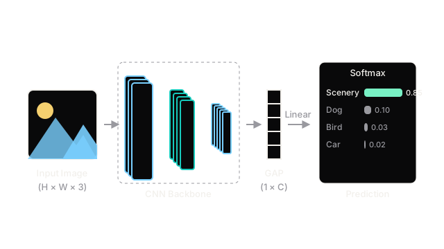
A CNN classifier has three parts:

1. Feature extractor (CNN backbone): A stack of convolution + ReLU + pooling layers transforms an input image of shape $H \times W \times 3$ into a feature map of shape $h \times w \times C$ . Each layer learns increasingly abstract patterns. Early layers detect edges; middle layers detect textures and parts; deep layers detect object-level structures.

2. Global average pooling (GAP): Reduces the spatial feature map to a vector of length $C$ by averaging each channel over spatial dimensions. Makes the classifier resolution-independent and reduces parameter count dramatically versus a flat fully-connected layer.

3. Classifier head: A single linear layer maps the $C$ -dimensional feature vector to $K$ class logits. A softmax converts logits to a probability distribution: $\hat{p}_k = \frac{e^{z_k}}{\sum_j e^{z_j}}$ .

Training objective

Cross-entropy loss between the predicted distribution $\hat{p}$ and the one-hot label $y$ :

$L = -\sum_{k=1}^{K} y_k \log \hat{p}_k = -\log \hat{p}_{y^*}$

Where $y^*$ is the true class index. Minimizing this is equivalent to maximizing the log probability of the correct class.

Evaluation metrics

Top-1 accuracy: The highest-probability class matches the label.
Top-5 accuracy: The true label is among the five highest-probability predictions. Used on ImageNet because multiple labels can be valid for an image (a photo of a labrador is also a dog).

Transfer learning

Training a ResNet-50 on ImageNet from scratch takes days on 8 GPUs. Most practitioners download pre-trained weights and fine-tune:

Feature extraction: freeze the backbone, train only the new head.
Fine-tuning: unfreeze the last few backbone layers and train with a small learning rate.

This works because early CNN layers learn universal features (edges, textures) that transfer across domains — medical images, satellite imagery, product photos.

Code

1import torch2from torchvision import models, transforms3from PIL import Image4
5# Load a pre-trained ResNet-50 (ImageNet weights)6model = models.resnet50(weights=models.ResNet50_Weights.IMAGENET1K_V2)7model.eval()8
9# Standard ImageNet preprocessing10preprocess = transforms.Compose([11    transforms.Resize(256),12    transforms.CenterCrop(224),13    transforms.ToTensor(),14    transforms.Normalize(mean=[0.485, 0.456, 0.406], std=[0.229, 0.224, 0.225]),15])16
17# Load and classify an image18image = Image.open("dog.jpg").convert("RGB")19input_tensor = preprocess(image).unsqueeze(0)  # add batch dimension: [1, 3, 224, 224]20
21with torch.no_grad():22    logits = model(input_tensor)23    probs = torch.softmax(logits, dim=1)24
25# Top-5 predictions26top5_probs, top5_idx = probs.topk(5)27print("Top-5 predictions:")28for prob, idx in zip(top5_probs[0], top5_idx[0]):29    print(f"  Class {idx.item():>4}: {prob.item():.3f}")30
31# Fine-tuning for a custom dataset (binary: cat vs dog)32num_classes = 233model.fc = torch.nn.Linear(model.fc.in_features, num_classes)  # replace head34
35# Freeze backbone, train only the new head36for param in model.parameters():37    param.requires_grad = False38for param in model.fc.parameters():39    param.requires_grad = True40
41optimizer = torch.optim.Adam(model.fc.parameters(), lr=1e-3)

Watch Out For

Shortcut learning and texture bias

CNNs trained on natural images learn texture shortcuts rather than shape features. A classifier can be fooled by adversarial examples that change textures imperceptibly to humans but dramatically to the model. Evaluate on augmented and out-of-distribution data to detect shortcut reliance before deployment.

Label distribution shift at test time

A classifier trained on 90% cats and 10% dogs will be confidently miscalibrated when deployed on a balanced dataset. The softmax probabilities are not reliable confidence scores out-of-the-box. Use temperature scaling or Platt scaling to calibrate predictions on the actual deployment distribution.

The Quick Version

Image classification assigns one class label to a fixed-size image from a predefined set.
Architecture: CNN feature extractor → global average pooling → linear + softmax.
Training minimizes cross-entropy loss; evaluation uses top-1 or top-5 accuracy.
AlexNet (2012) launched the deep learning era; ResNet (2015) solved the vanishing gradient problem that blocked very deep networks.
Transfer learning from ImageNet pre-trained weights dramatically reduces training time and data requirements for new domains.